Redis Stack was created to allow developers build to real-time applications with a back end data platform that can reliably process requests in under a millisecond. Redis Stack does this by extending Redis with modern data models and data processing tools (Document, Graph, Search, and Time Series).

Redis Stack unifies and simplifies the developer experience of the leading Redis modules and the capabilities they provide. Redis Stack bundles five Redis modules: RedisJSON, RedisSearch, RedisGraph, RedisTimeSeries, and RedisBloom.

Clients

Several Redis client libraries support Redis Stack. These include redis-py, node_redis, and Jedis. In addition, four higher-level object mapping libraries also support Redis Stack: Redis OM .NET, Redis OM Node, Redis OM Python, Redis OM Spring.

RedisInsight

Redis Stack also includes RedisInsight, a visualization tool for understanding and optimizing Redis data.

Redis Stack license

Redis Stack is made up of several components, licensed as follows:

Redis Stack Server combines open source Redis with RediSearch, RedisJSON RedisGraph, RedisTimeSeries and RedisBloom is licensed under the Redis Source Available License (RSAL).
RedisInsight is licensed under the Server Side Public License (SSPL).

1 - Get started with Redis Stack

How to install and get started with Redis Stack

1.1 - Install Redis Stack

How to install Redis Stack

1.1.1 - Install Redis Stack with binaries

How to install Redis Stack using tarballs

Start Redis Stack Server

After untarring or unzipping your redis-stack-server download, you can start Redis Stack Server as follows:

/path/to/redis-stack-server/bin/redis-stack-server

Add the binaries to your PATH

You can add the redis-stack-server binaries to your $PATH as follows:

Open the file ~/.bashrc or '~/zshrc` (depending on your shell), and add the following lines.

export PATH=/path/to/redis-stack-server/bin:$PATH

If you have an existing Redis installation on your system, then you can choose override those override those PATH variables as before, or you can choose to only add redis-stack-server binary as follows:

export PATH=/path/to/redis-stack-server/bin/redis-stack-server:$PATH

Now you can start Redis Stack Server as follows:

redis-stack-server

1.1.2 - Run Redis Stack on Docker

How to install Redis Stack using Docker

To get started with Redis Stack using Docker, you first need to select a Docker image:

redis/redis-stack contains both Redis Stack server and RedisInsight. This container is best for local development because you can use the embedded RedisInsight to visualize your data.
redis/redis-stack-server provides Redis Stack server only. This container is best for production deployment.

Getting started

redis/redis-stack-server

To start Redis Stack server using the redis-stack-server image, run the following command in your terminal:

docker run -d --name redis-stack-server -p 6379:6379 redis/redis-stack-server:latest

You can that the Redis Stack server database to your RedisInsight desktop applicaiton.

redis/redis-stack

To start Redis Stack developer container using the redis-stack image, run the following command in your terminal:

docker run -d --name redis-stack -p 6379:6379 -p 8001:8001 redis/redis-stack:latest

The docker run command above also exposes RedisInsight on port 8001. You can use RedisInsight by pointing your browser to http://localhost:8001.

Connect with redis-cli

You can then connect to the server using redis-cli, just as you connect to any Redis instance.

If you don’t have redis-cli installed locally, you can run it from the Docker container:

$ docker exec -it redis-stack redis-cli

Configuration

Persistence

To persist your Redis data to a local path, specify -v to configure a local volume. This command stores all data in the local directory local-data:

$ docker run -v /local-data/:/data redis/redis-stack:latest

Ports

If you want to expose Redis Stack server or RedisInsight on a different port, update the left hand of portion of the -p argument. This command exposes Redis Stack server on port 10001 and RedisInsight on port 13333:

$ docker run -p 10001:6379 -p 13333:8001 redis/redis-stack:latest

Config files

By default, the Redis Stack Docker containers use internal configuration files for Redis. To start Redis with local configuration file, you can use the -v volume options:

$ docker run -v `pwd`/local-redis-stack.conf:/redis-stack.conf -p 6379:6379 -p 8001:8001 redis/redis-stack:latest

Environment variables

To pass in arbitrary configuration changes, you can set any of these environment variables:

REDIS_ARGS: extra arguments for Redis
REDISEARCH_ARGS: arguments for RediSearch
REDISJSON_ARGS: arguments for RedisJSON
REDISGRAPH_ARGS: arguments for RedisGraph
REDISTIMESERIES_ARGS: arguments for RedisTimeSeries
REDISBLOOM_ARGS: arguments for RedisBloom

For example, here's how to use the REDIS_ARGS environment variable to pass the requirepass directive to Redis:

docker run -e REDIS_ARGS="--requirepass redis-stack" redis/redis-stack:latest

Here's how to set a retention policy for RedisTimeSeries:

docker run -e REDISTIMESERIES_ARGS="RETENTION_POLICY=20" redis/redis-stack:latest

1.1.3 - Install Redis Stack on Linux

How to install Redis Stack on Linux

From the official Debian/Ubuntu APT Repository

You can install recent stable versions of Redis Stack from the official packages.redis.io APT repository. The repository currently supports Ubuntu Xenial (16.04), Ubuntu Bionic (18.04), and Ubuntu Focal (20.04). Add the repository to the apt index, update it and install:

curl -fsSL https://packages.redis.io/gpg | sudo gpg --dearmor -o /usr/share/keyrings/redis-archive-keyring.gpg
echo "deb [signed-by=/usr/share/keyrings/redis-archive-keyring.gpg] https://packages.redis.io/deb $(lsb_release -cs) main" | sudo tee /etc/apt/sources.list.d/redis.list
sudo apt-get update
sudo apt-get install redis-stack-server

From the official offical RPM Feed

You can install recent stable versions of Redis Stack from the official packages.redis.io YUM repository. The repository currently supports RHEL7/CentOS7, and RHEL8/Centos8. Add the repository to the repository index, and install the package.

Create the file /etc/yum.repos.d/redis.repo with the following contents

[Redis]
name=Redis
baseurl=http://packages.redis.io/rpm/rhel7
enabled=1
gpgcheck=1

curl -fsSL https://packages.redis.io/gpg > /tmp/redis.key
sudo rpm --import /tmp/redis.key
sudo yum install epel-release
sudo yum install redis-stack-server

1.1.4 - Install Redis Stack on macOS

How to install Redis Stack on macOS

To install Redis Stack on macOS, use Homebrew. Make sure that you have Homebrew installed before starting on the installation instructions below.

There are three brew casks available.

redis-stack contains both redis-stack-server and redis-stack-redisinsight casks.
redis-stack-server provides Redis Stack server only.
redis-stack-redisinsight contains RedisInsight.

Install using Homebrew

First, tap the Redis Stack Homebrew tap:

brew tap redis-stack/redis-stack

Next, run brew install:

brew install redis-stack

The redis-stack-server cask will install all Redis and Redis Stack binaries. How you run these binaries depends on whether you already have Redis installed on your system.

First-time Redis installation

If this is the first time you've installed Redis on your system, then all Redis Stack binaries be installed and accessible from the $PATH. On M1 Macs, this assumes that /opt/homebrew/bin is in your path. On Intel-based Macs, /usr/local/bin should be in the $PATH.

To check this, run:

echo $PATH

Then, confirm that the output contains /opt/homebrew/bin (M1 Mac) or /usr/local/bin (Intel Mac). If these directories are not in the output, see the "Existing Redis installation" instructions below.

Existing Redis installation

If you have an existing Redis installation on your system, then might want to modify your $PATH to ensure that you're using the latest Redis Stack binaries.

Open the file ~/.bashrc or '~/zshrc` (depending on your shell), and add the following lines.

For Intel-based Macs:

export PATH=/usr/local/Caskroom/redis-stack-server/<VERSION>/bin:$PATH

For M1 Macs:

export PATH=/opt/homebrew/Caskroom/redis-stack-server/<VERSION>/bin:$PATH

In both cases, replace <VERSION> with your version of Redis Stack. For example, with version 6.2.0, path is as follows:

export PATH=/opt/homebrew/Caskroom/redis-stack-server/6.2.0/bin:$PATH

Start Redis Stack Server

You can now start Redis Stack Server as follows:

redis-stack-server

Installing Redis after installing Redis Stack

If you've already installed Redis Stack with Homebrew and then try to install Redis with brew install redis, you may encounter errors like the following:

Error: The brew link step did not complete successfully
The formula built, but is not symlinked into /usr/local
Could not symlink bin/redis-benchmark
Target /usr/local/bin/redis-benchmark
already exists. You may want to remove it:
rm '/usr/local/bin/redis-benchmark'

To force the link and overwrite all conflicting files:
brew link --overwrite redis

To list all files that would be deleted:
brew link --overwrite --dry-run redis

In this case, you can overwrite the Redis binaries installed by Redis Stack by running:

brew link --overwrite redis

However, Redis Stack Server will still be installed. To uninstall Redis Stack Server, see below.

Uninstall Redis Stack

To uninstall Redis Stack, run:

brew uninstall redis-stack-redisinsight redis-stack-server redis-stack
brew untap redis-stack/redis-stack

1.2 - Redis Stack clients

Client libraries supporting Redis Stack

Redis Stack is built on Redis and uses the same client protocol as Redis. As a result, most Redis client libraries work with Redis Stack. But some client libraries provide a more complete developer experience.

To meaningfully support Redis Stack support, a client library must provide an API for the commands exposed by Redis Stack. Core client libraries generally provide one method per Redis Stack command. High-level libraries provide abstractions that may make use of multiple commands.

Core client libraries

The following core client libraries support Redis Stack:

Jedis >= 4.0
node-redis >= 4.0
redis-py >= 4.0

High-level client libraries

The Redis OM client libraries let you use the document modeling, indexing, and querying capabilities of Redis Stack much like the way you'd use an ORM. The following Redis OM libraries support Redis Stack:

1.3 - Redis Stack tutorials

Learn how to write code against Redis Stack

1.3.1 - Redis OM .NET

Learn how to build with Redis Stack and .NET

Redis OM .NET is a purpose-built library for handling documents in Redis Stack. In this tutorial, we'll build a simple ASP.NET Core Web-API app for performing CRUD operations on a simple Person & Address model, and we'll accomplish all of this with Redis OM .NET.

Prerequisites

.NET 6 SDK
And IDE for writing .NET (Visual Studio, Rider, Visual Studio Code)
Optional: Docker Desktop for running redis-stack in docker for local testing.

If you want to skip this tutorial and just jump straight into code, all the source code is available in GitHub

Run Redis Stack

There are a variety of ways to run Redis Stack. One way is to use the docker image:

docker run -d -p 6379:6379 -p 8001:8001 redis/redis-stack

Create the project

To create the project, just run:

dotnet new webapi -n Redis.OM.Skeleton --no-https --kestrelHttpPort 5000

Then open the Redis.OM.Skeleton.csproj file in your IDE of choice.

Configure the app

Add a "REDIS_CONNECTION_STRING" field to your appsettings.jsonfile to configure the application. Set that connection string to be the URI of your Redis instance. If using the docker command mentioned earlier, your connection string will beredis://localhost:6379`.

Create the model

Now it's time to create the Person/Address model that the app will use for storing/retrieving people. Create a new directory called Model and add the files Address.cs and Person.cs to it. In Address.cs, add the following:

using Redis.OM.Modeling;

namespace Redis.OM.Skeleton.Model;

public class Address
{
    [Indexed]
    public int? StreetNumber { get; set; }
    
    [Indexed]
    public string? Unit { get; set; }
    
    [Searchable]
    public string? StreetName { get; set; }
    
    [Indexed]
    public string? City { get; set; }
    
    [Indexed]
    public string? State { get; set; }
    
    [Indexed]
    public string? PostalCode { get; set; }
    
    [Indexed]
    public string? Country { get; set; }
    
    [Indexed]
    public GeoLoc Location { get; set; }
}

Here, you'll notice that except StreetName, marked as Searchable, all the fields are decorated with the Indexed attribute. These attributes (Searchable and Indexed) tell Redis OM that you want to be able to use those fields in queries when querying your documents in Redis Stack. Address will not be a Document itself, so the top-level class is not decorated with anything; instead, the Address model will be embedded in our Person model.

To that end, add the following to Person.cs

using Redis.OM.Modeling;

namespace Redis.OM.Skeleton.Model;

[Document(StorageType = StorageType.Json, Prefixes = new []{"Person"})]
public class Person
{    
    [RedisIdField] [Indexed]public string? Id { get; set; }
    
    [Indexed] public string? FirstName { get; set; }

    [Indexed] public string? LastName { get; set; }
    
    [Indexed] public int Age { get; set; }
    
    [Searchable] public string? PersonalStatement { get; set; }
    
    [Indexed] public string[] Skills { get; set; } = Array.Empty<string>();    
    
    [Indexed(CascadeDepth = 1)] Address? Address { get; set; }
    
}

There are a few things to take note of here:

[Document(StorageType = StorageType.Json, Prefixes = new []{"Person"})] Indicates that the data type that Redis OM will use to store the document in Redis is JSON and that the prefix for the keys for the Person class will be Person.
[Indexed(CascadeDepth = 1)] Address? Address { get; set; } is one of two ways you can index an embedded object with Redis OM. This way instructs the index to cascade to the objects in the object graph, CascadeDepth of 1 means that it will traverse just one level, indexing the object as if it were building the index from scratch. The other method uses the JsonPath property of the individual indexed fields you want to search for. This more surgical approach limits the size of the index.
the Id property is marked as a RedisIdField. This denotes the field as one that will be used to generate the document's key name when it's stored in Redis.

Create the Index

With the model built, the next step is to create the index in Redis. The most correct way to manage this is to spin the index creation out into a Hosted Service, which will run which the app spins up. Create a' HostedServices' directory and add IndexCreationService.cs to that. In that file, add the following, which will create the index on startup.

using Redis.OM.Skeleton.Model;

namespace Redis.OM.Skeleton.HostedServices;

public class IndexCreationService : IHostedService
{
    private readonly RedisConnectionProvider _provider;
    public IndexCreationService(RedisConnectionProvider provider)
    {
        _provider = provider;
    }
    
    public async Task StartAsync(CancellationToken cancellationToken)
    {
        await _provider.Connection.CreateIndexAsync(typeof(Person));
    }

    public Task StopAsync(CancellationToken cancellationToken)
    {
        return Task.CompletedTask;
    }
}

Inject the RedisConnectionProvider

Redis OM uses the RedisConnectionProvider class to handle connections to Redis and provides the classes you can use to interact with Redis. To use it, simply inject an instance of the RedisConnectionProvider into your app. In your Program.cs file, add:

builder.Services.AddSingleton(new RedisConnectionProvider(builder.Configuration["REDIS_CONNECTION_STRING"]));

This will pull your connection string out of the config and initialize the provider. The provider will now be available in your controllers/services to use.

Create the PeopleController

The final puzzle piece is to write the actual API controller for our People API. In the controllers directory, add the file PeopleController.cs, the skeleton of the PeopleControllerclass will be:

using Microsoft.AspNetCore.Mvc;
using Redis.OM.Searching;
using Redis.OM.Skeleton.Model;

namespace Redis.OM.Skeleton.Controllers;

[ApiController]
[Route("[controller]")]
public class PeopleController : ControllerBase
{

}

Inject the RedisConnectionProvider

To interact with Redis, inject the RedisConnectionProvider. During this dependency injection, pull out a RedisCollection<Person> instance, which will allow a fluent interface for querying documents in Redis.

private readonly RedisCollection<Person> _people;
private readonly RedisConnectionProvider _provider;
public PeopleController(RedisConnectionProvider provider)
{
    _provider = provider;
    _people = (RedisCollection<Person>)provider.RedisCollection<Person>();
}

Add route for creating a Person

The first route to add to the API is a POST request for creating a person, using the RedisCollection, it's as simple as calling InsertAsync, passing in the person object:

[HttpPost]
public async Task<Person> AddPerson([FromBody] Person person)
{
    await _people.InsertAsync(person);
    return person;
}

Add route to filter by age

The first filter route to add to the API will let the user filter by a minimum and maximum age. Using the LINQ interface available to the RedisCollection, this is a simple operation:

[HttpGet("filterAge")]
public IList<Person> FilterByAge([FromQuery] int minAge, [FromQuery] int maxAge)
{        
    return _people.Where(x => x.Age >= minAge && x.Age <= maxAge).ToList();
}

Filter by GeoLocation

Redis OM has a GeoLoc data structure, an instance of which is indexed by the Address model, with the RedisCollection, it's possible to find all objects with a radius of particular position using the GeoFilter method along with the field you want to filter:

[HttpGet("filterGeo")]
public IList<Person> FilterByGeo([FromQuery] double lon, [FromQuery] double lat, [FromQuery] double radius, [FromQuery] string unit)
{
    return _people.GeoFilter(x => x.Address!.Location, lon, lat, radius, Enum.Parse<GeoLocDistanceUnit>(unit)).ToList();
}

Filter by exact string

When a string property in your model is marked as Indexed, e.g. FirstName and LastName, Redis OM can perform exact text matches against them. For example, the following two routes filter by PostalCode and name demonstrate exact string matches.

[HttpGet("filterName")]
public IList<Person> FilterByName([FromQuery] string firstName, [FromQuery] string lastName)
{
    return _people.Where(x => x.FirstName == firstName && x.LastName == lastName).ToList();
}

[HttpGet("postalCode")]
public IList<Person> FilterByPostalCode([FromQuery] string postalCode)
{
    return _people.Where(x => x.Address!.PostalCode == postalCode).ToList();
}

Filter with a full-text search

When a property in the model is marked as Searchable, like StreetAddress and PersonalStatement, you can perform a full-text search, see the filters for the PersonalStatement and StreetAddress:

[HttpGet("fullText")]
public IList<Person> FilterByPersonalStatement([FromQuery] string text){
    return _people.Where(x => x.PersonalStatement == text).ToList();
}

[HttpGet("streetName")]
public IList<Person> FilterByStreetName([FromQuery] string streetName)
{
    return _people.Where(x => x.Address!.StreetName == streetName).ToList();
}

Filter by array membership

When a string array or list is marked as Indexed, Redis OM can filter all the records containing a given string using the Contains method of the array or list. For example, our Person model has a list of skills you can query by adding the following route.

[HttpGet("skill")]
public IList<Person> FilterBySkill([FromQuery] string skill)
{
    return _people.Where(x => x.Skills.Contains(skill)).ToList();
}

Updating a person

Updating a document in Redis Stack with Redis OM can be done by first materializing the person object, making your desired changes, and then calling Save on the collection. The collection is responsible for keeping track of updates made to entities materialized in it; therefore, it will track and apply any updates you make in it. For example, add the following route to update the age of a Person given their Id:

[HttpPatch("updateAge/{id}")]
public IActionResult UpdateAge([FromRoute] string id, [FromBody] int newAge)
{
    foreach (var person in _people.Where(x => x.Id == id))
    {
        person.Age = newAge;
    }
    _people.Save();
    return Accepted();
}

Delete a person

Deleting a document from Redis can be done with Unlink. All that's needed is to call Unlink, passing in the key name. Given an id, we can reconstruct the key name using the prefix and the id:

[HttpDelete("{id}")]
public IActionResult DeletePerson([FromRoute] string id)
{
    _provider.Connection.Unlink($"Person:{id}");
    return NoContent();
}

Run the app

All that's left to do now is to run the app and test it. You can do so by running dotnet run, the app is now exposed on port 5000, and there should be a swagger UI that you can use to play with the API at http://localhost:5000/swagger. There's a couple of scripts, along with some data files, to insert some people into Redis using the API in the GitHub repo

Viewing data in with Redis Insight

You can either install the Redis Insight GUI or use the Redis Insight GUI running on http://localhost:8001/.

You can view the data by following these steps:

Accept the EULA

Accept EULA

Click the Add Redis Database button

Add Redis Database Button

Enter your hostname and port name for your redis server. If you are using the docker image, this is localhost and 6379 and give your database an alias

Configure Redis Insight Database

Click Add Redis Database.

Resources

The source code for this tutorial can be found in GitHub.
To learn more about Redis OM you can check out the the guide on Redis Developer

1.3.2 - Redis OM for Node.js

Learn how to build with Redis Stack and Node.js

This tutorial will show you how to build an API using Node.js and Redis Stack.

We'll be using Express and Redis OM to do this, and we assume that you have a basic understanding of Express.

The API we'll be building is a simple and relatively RESTful API that reads, writes, and finds data on persons: first name, last name, age, etc. We'll also add a simple location tracking feature just for a bit of extra interest.

But before we start with the coding, let's start with a description of what Redis OM is.

Redis OM for Node.js

Redis OM (pronounced REDiss OHM) is a library that provides object mapping for Redis—that's what the OM stands for... object mapping. It maps Redis data types — specifically Hashes and JSON documents — to JavaScript objects. And it allows you to search over these Hashes and JSON documents. It uses RedisJSON and RediSearch to do this.

RedisJSON and RediSearch are two of the modules included in Redis Stack. Modules are extensions to Redis that add new data types and new commands. RedisJSON adds a JSON document data type and the commands to manipulate it. RediSearch adds various search commands to index the contents of JSON documents and Hashes.

Redis OM comes in four different versions. We'll be working with Redis OM for Node.js in this tutorial, but there are also flavors and tutorials for Python, .NET, and Spring.

This tutorial will get you started with Redis OM for Node.js, covering the basics. But if you want to dive deep into all of Redis OM's capabilities, check out the README over on GitHub.

Prerequisites

Like anything software-related, you need to have some dependencies installed before you can get started:

Node.js 14.8+: In this tutorial, we're using JavaScript's top-level await feature which was introduced in Node 14.8. So, make sure you are using that version or later.
Redis Stack: You need a version of Redis Stack, either running locally on your machine or in the cloud.
RedisInsight: We'll use this to look inside Redis and make sure our code is doing what we think it's doing.

Starter code

We're not going to code this completely from scratch. Instead, we've provided some starter code for you. Go ahead and clone it to a folder of your convenience:

git clone git@github.com:redis-developer/express-redis-om-workshop.git

Now that you have the starter code, let's explore it a bit. Opening up server.js in the root we see that we have a simple Express app that uses Dotenv for configuration and Swagger UI Express for testing our API:

import 'dotenv/config'

import express from 'express'
import swaggerUi from 'swagger-ui-express'
import YAML from 'yamljs'

/* create an express app and use JSON */
const app = new express()
app.use(express.json())

/* set up swagger in the root */
const swaggerDocument = YAML.load('api.yaml')
app.use('/', swaggerUi.serve, swaggerUi.setup(swaggerDocument))

/* start the server */
app.listen(8080)

Alongside this is api.yaml, which defines the API we're going to build and provides the information Swagger UI Express needs to render its UI. You don't need to mess with it unless you want to add some additional routes.

The persons folder has some JSON files and a shell script. The JSON files are sample persons—all musicians because fun—that you can load into the API to test it. The shell script—load-data.sh—will load all the JSON files into the API using curl.

There are two empty folders, om and routers. The om folder is where all the Redis OM code will go. The routers folder will hold code for all of our Express routes.

Configure and run

The starter code is perfectly runnable if a bit thin. Let's configure and run it to make sure it works before we move on to writing actual code. First, get all the dependencies:

npm install

Then, set up a .env file in the root that Dotenv can make use of. There's a sample.env file in the root that you can copy and modify:

cp sample.env .env

The contents of .env looks like this:

# Put your local Redis Stack URL here. Want to run in the
# cloud instead? Sign up at https://redis.com/try-free/.
REDIS_URL=redis://localhost:6379

There's a good chance this is already correct. However, if you need to change the REDIS_URL for your particular environment (e.g., you're running Redis Stack in the cloud), this is the time to do it. Once done, you should be able to run the app:

npm start

Navigate to http://localhost:8080 and check out the client that Swagger UI Express has created. None of it works yet because we haven't implemented any of the routes. But, you can try them out and watch them fail!

The starter code runs. Let's add some Redis OM to it so it actually does something!

Setting up a Client

First things first, let's set up a client. The Client class is the thing that knows how to talk to Redis on behalf of Redis OM. One option is to put our client in its own file and export it. This ensures that the application has one and only one instance of Client and thus only one connection to Redis Stack. Since Redis and JavaScript are both (more or less) single-threaded, this works neatly.

Let's create our first file. In the om folder add a file called client.js and add the following code:

import { Client } from 'redis-om'

/* pulls the Redis URL from .env */
const url = process.env.REDIS_URL

/* create and open the Redis OM Client */
const client = await new Client().open(url)

export default client

Remember that top-level await stuff we mentioned earlier? There it is!

Note that we are getting our Redis URL from an environment variable. It was put there by Dotenv and read from our .env file. If we didn't have the .env file or have a REDIS_URL property in our .env file, this code would gladly read this value from the actual environment variables.

Also note that the .open() method conveniently returns this. This this (can I say this again? I just did!) lets us chain the instantiation of the client with the opening of the client. If this isn't to your liking, you could always write it like this:

/* create and open the Redis OM Client */
const client = new Client()
await client.open(url)

Entity, Schema, and Repository

Now that we have a client that's connected to Redis, we need to start mapping some persons. To do that, we need to define an Entity and a Schema. Let's start by creating a file named person.js in the om folder and importing client from client.js and the Entity and Schema classes from Redis OM:

import { Entity, Schema } from 'redis-om'
import client from './client.js'

Entity

Next, we need to define an entity. An Entity is the class that holds you data when you work with it—the thing being mapped to. It is what you create, read, update, and delete. Any class that extends Entity is an entity. We'll define our Person entity with a single line:

/* our entity */
class Person extends Entity {}

Schema

A schema defines the fields on your entity, their types, and how they are mapped internally to Redis. By default, entities map to JSON documents. Let's create our Schema in person.js:

/* create a Schema for Person */
const personSchema = new Schema(Person, {
  firstName: { type: 'string' },
  lastName: { type: 'string' },
  age: { type: 'number' },
  verified: { type: 'boolean' },
  location: { type: 'point' },
  locationUpdated: { type: 'date' },
  skills: { type: 'string[]' },
  personalStatement: { type: 'text' }
})

When you create a Schema, it modifies the Entity class you handed it (Person in our case) adding getters and setters for the properties you define. The type those getters and setters accept and return are defined with the type parameter as shown above. Valid values are: string, number, boolean, string[], date, point, and text.

The first three do exactly what you think—they define a property that is a String, a Number, or a Boolean. string[] does what you'd think as well, specifically defining an Array of strings.

date is a little different, but still more or less what you'd expect. It defines a property that returns a Date and can be set using not only a Date but also a String containing an ISO 8601 date or a Number with the UNIX epoch time in milliseconds.

A point defines a point somewhere on the globe as a longitude and a latitude. It creates a property that returns and accepts a simple object with the properties of longitude and latitude. Like this:

let point = { longitude: 12.34, latitude: 56.78 }

A text field is a lot like a string. If you're just reading and writing objects, they are identical. But if you want to search on them, they are very, very different. We'll talk about search more later, but the tl;dr is that string fields can only be matched on their whole value—no partial matches—and are best for keys while text fields have full-text search enabled on them and are optimized for human-readable text.

Repository

Now we have all the pieces that we need to create a repository. A Repository is the main interface into Redis OM. It gives us the methods to read, write, and remove a specific Entity. Create a Repository in person.js and make sure it's exported as you'll need it when we start implementing out API:

/* use the client to create a Repository just for Persons */
export const personRepository = client.fetchRepository(personSchema)

We're almost done with setting up our repository. But we still need to create an index or we won't be able to search. We do that by calling .createIndex(). If an index already exists and it's identical, this function won't do anything. If it's different, it'll drop it and create a new one. Add a call to .createIndex() to person.js:

/* create the index for Person */
await personRepository.createIndex()

That's all we need for person.js and all we need to start talking to Redis using Redis OM. Here's the code in its entirety:

import { Entity, Schema } from 'redis-om'
import client from './client.js'

/* our entity */
class Person extends Entity {}

/* create a Schema for Person */
const personSchema = new Schema(Person, {
  firstName: { type: 'string' },
  lastName: { type: 'string' },
  age: { type: 'number' },
  verified: { type: 'boolean' },
  location: { type: 'point' },
  locationUpdated: { type: 'date' },
  skills: { type: 'string[]' },
  personalStatement: { type: 'text' }
})

/* use the client to create a Repository just for Persons */
export const personRepository = client.fetchRepository(personSchema)

/* create the index for Person */
await personRepository.createIndex()

Now, let's add some routes in Express.

Set up the Person Router

Let's create a truly RESTful API with the CRUD operations mapping to PUT, GET, POST, and DELETE respectively. We're going to do this using Express Routers as this makes our code nice and tidy. Create a file called person-router.js in the routers folder and in it import Router from Express and personRepository from person.js. Then create and export a Router:

import { Router } from 'express'
import { personRepository } from '../om/person.js'

export const router = Router()

Imports and exports done, let's bind the router to our Express app. Open up server.js and import the Router we just created:

/* import routers */
import { router as personRouter } from './routers/person-router.js'

Then add the personRouter to the Express app:

/* bring in some routers */
app.use('/person', personRouter)

Your server.js should now look like this:

import 'dotenv/config'

import express from 'express'
import swaggerUi from 'swagger-ui-express'
import YAML from 'yamljs'

/* import routers */
import { router as personRouter } from './routers/person-router.js'

/* create an express app and use JSON */
const app = new express()
app.use(express.json())

/* bring in some routers */
app.use('/person', personRouter)

/* set up swagger in the root */
const swaggerDocument = YAML.load('api.yaml')
app.use('/', swaggerUi.serve, swaggerUi.setup(swaggerDocument))

/* start the server */
app.listen(8080)

Now we can add our routes to create, read, update, and delete persons. Head back to the person-router.js file so we can do just that.

Creating a Person

We'll create a person first as you need to have persons in Redis before you can do any of the reading, writing, or removing of them. Add the PUT route below. This route will call .createAndSave() to create a Person from the request body and immediately save it to the Redis:

router.put('/', async (req, res) => {
  const person = await personRepository.createAndSave(req.body)
  res.send(person)
})

Note that we are also returning the newly created Person. Let's see what that looks like by actually calling our API using the Swagger UI. Go to http://localhost:8080 in your browser and try it out. The default request body in Swagger will be fine for testing. You should see a response that looks like this:

{
  "entityId": "01FY9MWDTWW4XQNTPJ9XY9FPMN",
  "firstName": "Rupert",
  "lastName": "Holmes",
  "age": 75,
  "verified": false,
  "location": {
    "longitude": 45.678,
    "latitude": 45.678
  },
  "locationUpdated": "2022-03-01T12:34:56.123Z",
  "skills": [
    "singing",
    "songwriting",
    "playwriting"
  ],
  "personalStatement": "I like piña coladas and walks in the rain"
}

This is exactly what we handed it with one exception: the entityId. Every entity in Redis OM has an entity ID which is—as you've probably guessed—the unique ID of that entity. It was randomly generated when we called .createAndSave(). Yours will be different, so make note of it.

You can see this newly created JSON document in Redis with RedisInsight. Go ahead and launch RedisInsight and you should see a key with a name like Person:01FY9MWDTWW4XQNTPJ9XY9FPMN. The Person bit of the key was derived from the class name of our entity and the sequence of letters and numbers is our generated entity ID. Click on it to take a look at the JSON document you've created.

You'll also see a key named Person:index:hash. That's a unique value that Redis OM uses to see if it needs to recreate the index or not when .createIndex() is called. You can safely ignore it.

Reading a Person

Create down, let's add a GET route to read this newly created Person:

router.get('/:id', async (req, res) => {
  const person = await personRepository.fetch(req.params.id)
  res.send(person)
})

This code extracts a parameter from the URL used in the route—the entityId that we received previously. It uses the .fetch() method on the personRepository to retrieve a Person using that entityId. Then, it returns that Person.

Let's go ahead and test that in Swagger as well. You should get back exactly the same response. In fact, since this is a simple GET, we should be able to just load the URL into our browser. Test that out too by navigating to http://localhost:8080/person/01FY9MWDTWW4XQNTPJ9XY9FPMN, replacing the entity ID with your own.

Now that we can read and write, let's implement the REST of the HTTP verbs. REST... get it?

Updating a Person

Let's add the code to update a person using a POST route:

router.post('/:id', async (req, res) => {

  const person = await personRepository.fetch(req.params.id)

  person.firstName = req.body.firstName ?? null
  person.lastName = req.body.lastName ?? null
  person.age = req.body.age ?? null
  person.verified = req.body.verified ?? null
  person.location = req.body.location ?? null
  person.locationUpdated = req.body.locationUpdated ?? null
  person.skills = req.body.skills ?? null
  person.personalStatement = req.body.personalStatement ?? null

  await personRepository.save(person)

  res.send(person)
})

This code fetches the Person from the personRepository using the entityId just like our previous route did. However, now we change all the properties based on the properties in the request body. If any of them are missing, we set them to null. Then, we call .save() and return the changed Person.

Let's test this in Swagger too, why not? Make some changes. Try removing some of the fields. What do you get back when you read it after you've changed it?

Deleting a Person

Deletion—my favorite! Remember kids, deletion is 100% compression. The route that deletes is just as straightforward as the one that reads, but much more destructive:

router.delete('/:id', async (req, res) => {
  await personRepository.remove(req.params.id)
  res.send({ entityId: req.params.id })
})

I guess we should probably test this one out too. Load up Swagger and exercise the route. You should get back JSON with the entity ID you just removed:

{
  "entityId": "01FY9MWDTWW4XQNTPJ9XY9FPMN"
}

And just like that, it's gone!

All the CRUD

Do a quick check with what you've written so far. Here's what should be the totality of your person-router.js file:

import { Router } from 'express'
import { personRepository } from '../om/person.js'

export const router = Router()

router.put('/', async (req, res) => {
  const person = await personRepository.createAndSave(req.body)
  res.send(person)
})

router.get('/:id', async (req, res) => {
  const person = await personRepository.fetch(req.params.id)
  res.send(person)
})

router.post('/:id', async (req, res) => {

  const person = await personRepository.fetch(req.params.id)

  person.firstName = req.body.firstName ?? null
  person.lastName = req.body.lastName ?? null
  person.age = req.body.age ?? null
  person.verified = req.body.verified ?? null
  person.location = req.body.location ?? null
  person.locationUpdated = req.body.locationUpdated ?? null
  person.skills = req.body.skills ?? null
  person.personalStatement = req.body.personalStatement ?? null

  await personRepository.save(person)

  res.send(person)
})

router.delete('/:id', async (req, res) => {
  await personRepository.remove(req.params.id)
  res.send({ entityId: req.params.id })
})

Preparing to search

CRUD completed, let's do some searching. In order to search, we need data to search over. Remember that persons folder with all the JSON documents and the load-data.sh shell script? Its time has arrived. Go into that folder and run the script:

cd persons
./load-data.sh

You should get a rather verbose response containing the JSON response from the API and the names of the files you loaded. Like this:

{"entityId":"01FY9Z4RRPKF4K9H78JQ3K3CP3","firstName":"Chris","lastName":"Stapleton","age":43,"verified":true,"location":{"longitude":-84.495,"latitude":38.03},"locationUpdated":"2022-01-01T12:00:00.000Z","skills":["singing","football","coal mining"],"personalStatement":"There are days that I can walk around like I'm alright. And I pretend to wear a smile on my face. And I could keep the pain from comin' out of my eyes. But sometimes, sometimes, sometimes I cry."} <- chris-stapleton.json
{"entityId":"01FY9Z4RS2QQVN4XFYSNPKH6B2","firstName":"David","lastName":"Paich","age":67,"verified":false,"location":{"longitude":-118.25,"latitude":34.05},"locationUpdated":"2022-01-01T12:00:00.000Z","skills":["singing","keyboard","blessing"],"personalStatement":"I seek to cure what's deep inside frightened of this thing that I've become"} <- david-paich.json
{"entityId":"01FY9Z4RSD7SQMSWDFZ6S4M5MJ","firstName":"Ivan","lastName":"Doroschuk","age":64,"verified":true,"location":{"longitude":-88.273,"latitude":40.115},"locationUpdated":"2022-01-01T12:00:00.000Z","skills":["singing","dancing","friendship"],"personalStatement":"We can dance if we want to. We can leave your friends behind. 'Cause your friends don't dance and if they don't dance well they're no friends of mine."} <- ivan-doroschuk.json
{"entityId":"01FY9Z4RSRZFGQ21BMEKYHEVK6","firstName":"Joan","lastName":"Jett","age":63,"verified":false,"location":{"longitude":-75.273,"latitude":40.003},"locationUpdated":"2022-01-01T12:00:00.000Z","skills":["singing","guitar","black eyeliner"],"personalStatement":"I love rock n' roll so put another dime in the jukebox, baby."} <- joan-jett.json
{"entityId":"01FY9Z4RT25ABWYTW6ZG7R79V4","firstName":"Justin","lastName":"Timberlake","age":41,"verified":true,"location":{"longitude":-89.971,"latitude":35.118},"locationUpdated":"2022-01-01T12:00:00.000Z","skills":["singing","dancing","half-time shows"],"personalStatement":"What goes around comes all the way back around."} <- justin-timberlake.json
{"entityId":"01FY9Z4RTD9EKBDS2YN9CRMG1D","firstName":"Kerry","lastName":"Livgren","age":72,"verified":false,"location":{"longitude":-95.689,"latitude":39.056},"locationUpdated":"2022-01-01T12:00:00.000Z","skills":["poetry","philosophy","songwriting","guitar"],"personalStatement":"All we are is dust in the wind."} <- kerry-livgren.json
{"entityId":"01FY9Z4RTR73HZQXK83JP94NWR","firstName":"Marshal","lastName":"Mathers","age":49,"verified":false,"location":{"longitude":-83.046,"latitude":42.331},"locationUpdated":"2022-01-01T12:00:00.000Z","skills":["rapping","songwriting","comics"],"personalStatement":"Look, if you had, one shot, or one opportunity to seize everything you ever wanted, in one moment, would you capture it, or just let it slip?"} <- marshal-mathers.json
{"entityId":"01FY9Z4RV2QHH0Z1GJM5ND15JE","firstName":"Rupert","lastName":"Holmes","age":75,"verified":true,"location":{"longitude":-2.518,"latitude":53.259},"locationUpdated":"2022-01-01T12:00:00.000Z","skills":["singing","songwriting","playwriting"],"personalStatement":"I like piña coladas and taking walks in the rain."} <- rupert-holmes.json

A little messy, but if you don't see this, then it didn't work!

Now that we have some data, let's add another router to hold the search routes we want to add. Create a file named search-router.js in the routers folder and set it up with imports and exports just like we did in person-router.js:

import { Router } from 'express'
import { personRepository } from '../om/person.js'

export const router = Router()

Import the Router into server.js the same way we did for the personRouter:

/* import routers */
import { router as personRouter } from './routers/person-router.js'
import { router as searchRouter } from './routers/search-router.js'

Then add the searchRouter to the Express app:

/* bring in some routers */
app.use('/person', personRouter)
app.use('/persons', searchRouter)

Router bound, we can now add some routes.

Search all the things

We're going to add a plethora of searches to our new Router. But the first will be the easiest as it's just going to return everything. Go ahead and add the following code to search-router.js:

router.get('/all', async (req, res) => {
  const persons = await personRepository.search().return.all()
  res.send(persons)
})

Here we see how to start and finish a search. Searches start just like CRUD operations start—on a Repository. But instead of calling .createAndSave(), .fetch(), .save(), or .remove(), we call .search(). And unlike all those other methods, .search() doesn't end there. Instead, it allows you to build up a query (which you'll see in the next example) and then resolve it with a call to .return.all().

With this new route in place, go into the Swagger UI and exercise the /persons/all route. You should see all of the folks you added with the shell script as a JSON array.

In the example above, the query is not specified—we didn't build anything up. If you do this, you'll just get everything. Which is what you want sometimes. But not most of the time. It's not really searching if you just return everything. So let's add a route that lets us find persons by their last name. Add the following code:

router.get('/by-last-name/:lastName', async (req, res) => {
  const lastName = req.params.lastName
  const persons = await personRepository.search()
    .where('lastName').equals(lastName).return.all()
  res.send(persons)
})

In this route, we're specifying a field we want to filter on and a value that it needs to equal. The field name in the call to .where() is the name of the field specified in our schema. This field was defined as a string, which matters because the type of the field determines the methods that are available query it.

In the case of a string, there's just .equals(), which will query against the value of the entire string. This is aliased as .eq(), .equal(), and .equalTo() for your convenience. You can even add a little more syntactic sugar with calls to .is and .does that really don't do anything but make your code pretty. Like this:

const persons = await personRepository.search().where('lastName').is.equalTo(lastName).return.all()
const persons = await personRepository.search().where('lastName').does.equal(lastName).return.all()

You can also invert the query with a call to .not:

const persons = await personRepository.search().where('lastName').is.not.equalTo(lastName).return.all()
const persons = await personRepository.search().where('lastName').does.not.equal(lastName).return.all()

In all these cases, the call to .return.all() executes the query we build between it and the call to .search(). We can search on other field types as well. Let's add some routes to search on a number and a boolean field:

router.get('/old-enough-to-drink-in-america', async (req, res) => {
  const persons = await personRepository.search()
    .where('age').gte(21).return.all()
  res.send(persons)
})

router.get('/non-verified', async (req, res) => {
  const persons = await personRepository.search()
    .where('verified').is.not.true().return.all()
  res.send(persons)
})

The number field is filtering persons by age where the age is great than or equal to 21. Again, there are aliases and syntactic sugar:

const persons = await personRepository.search().where('age').is.greaterThanOrEqualTo(21).return.all()

But there are also more ways to query:

const persons = await personRepository.search().where('age').eq(21).return.all()
const persons = await personRepository.search().where('age').gt(21).return.all()
const persons = await personRepository.search().where('age').gte(21).return.all()
const persons = await personRepository.search().where('age').lt(21).return.all()
const persons = await personRepository.search().where('age').lte(21).return.all()
const persons = await personRepository.search().where('age').between(21, 65).return.all()

The boolean field is searching for persons by their verification status. It already has some of our syntactic sugar in it. Note that this query will match a missing value or a false value. That's why I specified .not.true(). You can also call .false() on boolean fields as well as all the variations of .equals.

const persons = await personRepository.search().where('verified').true().return.all()
const persons = await personRepository.search().where('verified').false().return.all()
const persons = await personRepository.search().where('verified').equals(true).return.all()

So, we've created a few routes and I haven't told you to test them. Maybe you have anyhow. If so, good for you, you rebel. For the rest of you, why don't you go ahead and test them now with Swagger? And, going forward, just test them when you want. Heck, create some routes of your own using the provided syntax and try those out too. Don't let me tell you how to live your life.

Of course, querying on just one field is never enough. Not a problem, Redis OM can handle .and() and .or() like in this route:

router.get('/verified-drinkers-with-last-name/:lastName', async (req, res) => {
  const lastName = req.params.lastName
  const persons = await personRepository.search()
    .where('verified').is.true()
      .and('age').gte(21)
      .and('lastName').equals(lastName).return.all()
  res.send(persons)
})

Here, I'm just showing the syntax for .and() but, of course, you can also use .or().

Full-text search

If you've defined a field with a type of text in your schema, you can perform full-text searches against it. The way a text field is searched is different from how a string is searched. A string can only be compared with .equals() and must match the entire string. With a text field, you can look for words within the string.

A text field is optimized for human-readable text, like an essay or song lyrices. It's pretty clever. It understands that certain words (like a, an, or the) are common and ignores them. It understands how words are grammatically similar and so if you search for give, it matches gives, given, giving, and gave too. And it ignores punctuation.

Let's add a route that does full-text search against our personalStatement field:

router.get('/with-statement-containing/:text', async (req, res) => {
  const text = req.params.text
  const persons = await personRepository.search()
    .where('personalStatement').matches(text)
      .return.all()
  res.send(persons)
})

Note the use of the .matches() function. This is the only one that works with text fields. It takes a string that can be one or more words—space-delimited—that you want to quyery for. Let's try it out. In Swagger, use this route to search for the word "walk". You should get the following results:

[
  {
    "entityId": "01FYC7CTR027F219455PS76247",
    "firstName": "Rupert",
    "lastName": "Holmes",
    "age": 75,
    "verified": true,
    "location": {
      "longitude": -2.518,
      "latitude": 53.259
    },
    "locationUpdated": "2022-01-01T12:00:00.000Z",
    "skills": [
      "singing",
      "songwriting",
      "playwriting"
    ],
    "personalStatement": "I like piña coladas and taking walks in the rain."
  },
  {
    "entityId": "01FYC7CTNBJD9CZKKWPQEZEW14",
    "firstName": "Chris",
    "lastName": "Stapleton",
    "age": 43,
    "verified": true,
    "location": {
      "longitude": -84.495,
      "latitude": 38.03
    },
    "locationUpdated": "2022-01-01T12:00:00.000Z",
    "skills": [
      "singing",
      "football",
      "coal mining"
    ],
    "personalStatement": "There are days that I can walk around like I'm alright. And I pretend to wear a smile on my face. And I could keep the pain from comin' out of my eyes. But sometimes, sometimes, sometimes I cry."
  }
]

Notice how the word "walk" is matched for Rupert Holmes' personal statement that contains "walks" and matched for Chris Stapleton's that contains "walk". Now search "walk raining". You'll see that this returns Rupert's entry only even though the exact text of neither of these words is found in his personal statement. But they are grammatically related so it matched them. This is called stemming and it's a pretty cool feature of RediSearch that Redis OM exploits.

And if you search for "a rain walk" you'll still match Rupert's entry even though the word "a" is not in the text. Why? Because it's a common word that's not very helpful with searching. These common words are called stop words and this is another cool feature of RediSearch that Redis OM just gets for free.

Searching the globe

RediSearch, and therefore Redis OM, both support searching by geographic location. You specify a point in the globe, a radius, and the units for that radius and it'll gleefully return all the entities therein. Let's add a route to do just that:

router.get('/near/:lng,:lat/radius/:radius', async (req, res) => {
  const longitude = Number(req.params.lng)
  const latitude = Number(req.params.lat)
  const radius = Number(req.params.radius)

  const persons = await personRepository.search()
    .where('location')
      .inRadius(circle => circle
          .longitude(longitude)
          .latitude(latitude)
          .radius(radius)
          .miles)
        .return.all()

  res.send(persons)
})

This code looks a little different than the others because the way we define the circle we want to search is done with a function that is passed into the .inRadius method:

circle => circle.longitude(longitude).latitude(latitude).radius(radius).miles

All this function does is accept an instance of a Circle that has been initialized with default values. We override those values by calling various builder methods to define the origin of our search (i.e. the longitude and latitude), the radius, and the units that radius is measured in. Valid units are miles, meters, feet, and kilometers.

Let's try the route out. I know we can find Joan Jett at around longitude -75.0 and latitude 40.0, which is in eastern Pennsylvania. So use those coordinates with a radius of 20 miles. You should receive in response:

[
  {
    "entityId": "01FYC7CTPKYNXQ98JSTBC37AS1",
    "firstName": "Joan",
    "lastName": "Jett",
    "age": 63,
    "verified": false,
    "location": {
      "longitude": -75.273,
      "latitude": 40.003
    },
    "locationUpdated": "2022-01-01T12:00:00.000Z",
    "skills": [
      "singing",
      "guitar",
      "black eyeliner"
    ],
    "personalStatement": "I love rock n' roll so put another dime in the jukebox, baby."
  }
]

Try widening the radius and see who else you can find.

Adding location tracking

We're getting toward the end of the tutorial here, but before we go, I'd like to add that location tracking piece that I mentioned way back in the beginning. This next bit of code should be easily understood if you've gotten this far as it's not really doing anything I haven't talked about already.

Add a new file called location-router.js in the routers folder:

import { Router } from 'express'
import { personRepository } from '../om/person.js'

export const router = Router()

router.patch('/:id/location/:lng,:lat', async (req, res) => {

  const id = req.params.id
  const longitude = Number(req.params.lng)
  const latitude = Number(req.params.lat)

  const locationUpdated = new Date()

  const person = await personRepository.fetch(id)
  person.location = { longitude, latitude }
  person.locationUpdated = locationUpdated
  await personRepository.save(person)

  res.send({ id, locationUpdated, location: { longitude, latitude } })
})

Here we're calling .fetch() to fetch a person, we're updating some values for that person—the .location property with our longitude and latitude and the .locationUpdated property with the current date and time. Easy stuff.

To use this Router, import it in server.js:

/* import routers */
import { router as personRouter } from './routers/person-router.js'
import { router as searchRouter } from './routers/search-router.js'
import { router as locationRouter } from './routers/location-router.js'

And bind the router to a path:

/* bring in some routers */
app.use('/person', personRouter, locationRouter)
app.use('/persons', searchRouter)

And that's that. But this just isn't enough to satisfy. It doesn't show you anything new, except maybe the usage of a date field. And, it's not really location tracking. It just shows where these people last were, no history. So let's add some!.

To add some history, we're going to use a Redis Stream. Streams are a big topic but don't worry if you’re not familiar with them, you can think of them as being sort of like a log file stored in a Redis key where each entry represents an event. In our case, the event would be the person moving about or checking in or whatever.

But there's a problem. Redis OM doesn’t support Streams even though Redis Stack does. So how do we take advantage of them in our application? By using Node Redis. Node Redis is a low-level Redis client for Node.js that gives you access to all the Redis commands and data types. Internally, Redis OM is creating and using a Node Redis connection. You can use that connection too. Or rather, Redis OM can be told to use the connection you are using. Let me show you how.

Using Node Redis

Open up client.js in the om folder. Remember how we created a Redis OM Client and then called .open() on it?

const client = await new Client().open(url)

Well, the Client class also has a .use() method that takes a Node Redis connection. Modify client.js to open a connection to Redis using Node Redis and then .use() it:

import { Client } from 'redis-om'
import { createClient } from 'redis'

/* pulls the Redis URL from .env */
const url = process.env.REDIS_URL

/* create a connection to Redis with Node Redis */
export const connection = createClient({ url })
await connection.connect()

/* create a Client and bind it to the Node Redis connection */
const client = await new Client().use(connection)

export default client

And that's it. Redis OM is now using the connection you created. Note that we are exporting both the client and the connection. Got to export the connection if we want to use it in our newest route.

Storing location history with Streams

To add an event to a Stream we need to use the XADD command. Node Redis exposes that as .xAdd(). So, we need to add a call to .xAdd() in our route. Modify location-router.js to import our connection:

import { connection } from '../om/client.js'

And then in the route itself add a call to .xAdd():

  ...snip...
  const person = await personRepository.fetch(id)
  person.location = { longitude, latitude }
  person.locationUpdated = locationUpdated
  await personRepository.save(person)

  let keyName = `${person.keyName}:locationHistory`
  await connection.xAdd(keyName, '*', person.location)
  ...snip...

.xAdd() takes a key name, an event ID, and a JavaScript object containing the keys and values that make up the event, i.e. the event data. For the key name, we're building a string using the .keyName property that Person inherited from Entity (which will return something like Peson:01FYC7CTPKYNXQ98JSTBC37AS1) combined with a hard-coded value. We're passing in * for our event ID, which tells Redis to just generate it based on the current time and previous event ID. And we're passing in the location—with properties of longitude and latitude—as our event data.

Now, whenever this route is exercised, the longitude and latitude will be logged and the event ID will encode the time. Go ahead and use Swagger to move Joan Jett around a few times.

Now, go into RedisInsight and take a look at the Stream. You'll see it there in the list of keys but if you click on it, you'll get a message saying that "This data type is coming soon!". If you don't get this message, congratualtions, you live in the future! For us here in the past, we'll just issue the raw command instead:

XRANGE Person:01FYC7CTPKYNXQ98JSTBC37AS1:locationHistory - +

This tells Redis to get a range of values from a Stream stored in the given the key name—Person:01FYC7CTPKYNXQ98JSTBC37AS1:locationHistory in our example. The next values are the starting event ID and the ending event ID. - is the beginning of the Stream. + is the end. So this returns everything in the Stream:

1) 1) "1647536562911-0"
  2) 1) "longitude"
      2) "45.678"
      3) "latitude"
      4) "45.678"
2) 1) "1647536564189-0"
  2) 1) "longitude"
      2) "45.679"
      3) "latitude"
      4) "45.679"
3) 1) "1647536565278-0"
  2) 1) "longitude"
      2) "45.680"
      3) "latitude"
      4) "45.680"

And just like that, we're tracking Joan Jett.

Wrap-up

So, now you know how to use Express + Redis OM to build an API backed by Redis Stack. And, you've got yourself some pretty decent started code in the process. Good deal! If you want to learn more, you can check out the documentation for Redis OM. It covers the full breadth of Redis OM's capabilities.

And thanks for taking the time to work through this. I sincerly hope you found it useful. If you have any questions, the Redis Discord server is by far the best place to get them answered. Join the server and ask away!

1.3.3 - Redis OM Python

Learn how to build with Redis Stack and Python

Redis OM Python is a Redis client that provides high-level abstractions for managing document data in Redis. This tutorial shows you how to get up and running with Redis OM Python, Redis Stack, and the Flask micro-framework.

We'd love to see what you build with Redis Stack and Redis OM. Join the Redis community on Discord to chat with us about all things Redis OM and Redis Stack. Read more about Redis OM Python our announcement blog post.

Overview

This application, an API built with Flask and a simple domain model, demonstrates common data manipulation patterns using Redis OM.

Our entity is a Person, with the following JSON representation:

{
  "first_name": "A string, the person's first or given name",
  "last_name": "A string, the person's last or surname",
  "age": 36,
  "address": {
    "street_number": 56,
    "unit": "A string, optional unit number e.g. A or 1",
    "street_name": "A string, name of the street they live on",
    "city": "A string, name of the city they live in",
    "state": "A string, state, province or county that they live in",
    "postal_code": "A string, their zip or postal code",
    "country": "A string, country that they live in."
  },
  "personal_statement": "A string, free text personal statement",
  "skills": [
    "A string: a skill the person has",
    "A string: another still that the person has"
  ]
}

We'll let Redis OM handle generation of unique IDs, which it does using ULIDs. Redis OM will also handle creation of unique Redis key names for us, as well as saving and retrieving entities from JSON documents stored in a Redis Stack database.

Getting Started

Requirements

To run this application you'll need:

git - to clone the repo to your machine.
Python 3.9 or higher.
A Redis Stack database, or Redis with the RediSearch and RedisJSON modules installed. We've provided a docker-compose.yml for this. You can also sign up for a free 30Mb database with Redis Enterprise Cloud - be sure to check the Redis Stack option when creating your cloud database.
curl, or Postman - to send HTTP requests to the application. We'll provide examples using curl in this document.
Optional: RedisInsight, a free data visualization and database management tool for Redis. When downloading RedisInsight, be sure to select version 2.x or use the version that comes with Redis Stack.

Get the Source Code

Clone the repository from GitHub:

$ git clone https://github.com/redis-developer/redis-om-python-flask-skeleton-app.git
$ cd redis-om-python-flask-skeleton-app

Start a Redis Stack Database, or Configure your Redis Enterprise Cloud Credentials

Next, we'll get a Redis Stack database up and running. If you're using Docker:

$ docker-compose up -d
Creating network "redis-om-python-flask-skeleton-app_default" with the default driver
Creating redis_om_python_flask_starter ... done

If you're using Redis Enterprise Cloud, you'll need the hostname, port number, and password for your database. Use these to set the REDIS_OM_URL environment variable like this:

$ export REDIS_OM_URL=redis://default:<password>@<host>:<port>

(This step is not required when working with Docker as the Docker container runs Redis on localhost port 6379 with no password, which is the default connection that Redis OM uses.)

For example if your Redis Enterprise Cloud database is at port 9139 on host enterprise.redis.com and your password is 5uper53cret then you'd set REDIS_OM_URL as follows:

$ export REDIS_OM_URL=redis://default:5uper53cret@enterprise.redis.com:9139

Create a Python Virtual Environment and Install the Dependencies

Create a Python virtual environment, and install the project dependencies which are Flask, Requests (used only in the data loader script) and Redis OM:

$ python3 -m venv venv
$ . ./venv/bin/activate
$ pip install -r requirements.txt

Start the Flask Application

Let's start the Flask application in development mode, so that Flask will restart the server for you each time you save code changes in app.py:

$ export FLASK_ENV=development
$ flask run

If all goes well, you should see output similar to this:

$ flask run
 * Environment: development
 * Debug mode: on
 * Running on http://127.0.0.1:5000/ (Press CTRL+C to quit)
 * Restarting with stat
 * Debugger is active!
 * Debugger PIN: XXX-XXX-XXX

You're now up and running, and ready to perform CRUD operations on data with Redis, RediSearch, RedisJSON and Redis OM for Python! To make sure the server's running, point your browser at http://127.0.0.1:5000/, where you can expect to see the application's basic home page:

screenshot

Load the Sample Data

We've provided a small amount of sample data (it's in data/people.json. The Python script dataloader.py loads each person into Redis by posting the data to the application's create a new person endpoint. Run it like this:

$ python dataloader.py
Created person Robert McDonald with ID 01FX8RMR7NRS45PBT3XP9KNAZH
Created person Kareem Khan with ID 01FX8RMR7T60ANQTS4P9NKPKX8
Created person Fernando Ortega with ID 01FX8RMR7YB283BPZ88HAG066P
Created person Noor Vasan with ID 01FX8RMR82D091TC37B45RCWY3
Created person Dan Harris with ID 01FX8RMR8545RWW4DYCE5MSZA1

Make sure to take a copy of the output of the data loader, as your IDs will differ from those used in the tutorial. To follow along, substitute your IDs for the ones shown above. e.g. whenever we are working with Kareem Khan, change 01FX8RMR7T60ANQTS4P9NKPKX8 for the ID that your data loader assiged to Kareem in your Redis database.

Problems?

If the Flask server fails to start, take a look at its output. If you see log entries similar to this:

raise ConnectionError(self._error_message(e))
redis.exceptions.ConnectionError: Error 61 connecting to localhost:6379. Connection refused.

then you need to start the Redis Docker container if using Docker, or set the REDIS_OM_URL environment variable if using Redis Enterprise Cloud.

If you've set the REDIS_OM_URL environment variable, and the code errors with something like this on startup:

raise ConnectionError(self._error_message(e))
redis.exceptions.ConnectionError: Error 8 connecting to enterprise.redis.com:9139. nodename nor servname provided, or not known.

then you'll need to check that you used the correct hostname, port, password and format when setting REDIS_OM_URL.

If the data loader fails to post the sample data into the application, make sure that the Flask application is running before running the data loader.

Create, Read, Update and Delete Data

Let's create and manipulate some instances of our data model in Redis. Here we'll look at how to call the Flask API with curl (you could also use Postman), how the code works, and how the data's stored in Redis.

Building a Person Model with Redis OM

Redis OM allows us to model entities using Python classes, and the Pydantic framework. Our person model is contained in the file person.py. Here's some notes about how it works:

We declare a class Person which extends a Redis OM class JsonModel. This tells Redis OM that we want to store these entities in Redis as JSON documents.
We then declare each field in our model, specifying the data type and whether or not we want to index on that field. For example, here's the age field, which we've declared as a positive integer that we want to index on:

age: PositiveInt = Field(index=True)

The skills field is a list of strings, declared thus:

skills: List[str] = Field(index=True)

For the personal_statement field, we don't want to index on the field's value, as it's a free text sentence rather than a single word or digit. For this, we'll tell Redis OM that we want to be able to perform full text searches on the values:

personal_statement: str = Field(index=True, full_text_search=True)

address works differently from the other fields. Note that in our JSON representation of the model, address is an object rather than a string or numerical field. With Redis OM, this is modeled as a second class, which extends the Redis OM EmbeddedJsonModel class:

class Address(EmbeddedJsonModel):
    # field definitions...

Fields in an EmbeddedJsonModel are defined in the same way, so our class contains a field definition for each data item in the address.
Not every field in our JSON is present in every address, Redis OM allows us to declare a field as optional so long as we don't index it:

unit: Optional[str] = Field(index=False)

We can also set a default value for a field... let's say country should be "United Kingdom" unless otherwise specified:

country: str = Field(index=True, default="United Kingdom")

Finally, to add the embedded address object to our Person model, we declare a field of type Address in the Person class:

address: Address

Adding New People

The function create_person in app.py handles the creation of a new person in Redis. It expects a JSON object that adheres to our Person model's schema. The code to then create a new Person object with that data and save it in Redis is simple:

  new_person = Person(**request.json)
  new_person.save()
  return new_person.pk

When a new Person instance is created, Redis OM assigns it a unique ULID primary key, which we can access as .pk. We return that to the caller, so that they know the ID of the object they just created.

Persisting the object to Redis is then simply a matter of calling .save() on it.

Try it out... with the server running, add a new person using curl:

curl --location --request POST 'http://127.0.0.1:5000/person/new' \
--header 'Content-Type: application/json' \
--data-raw '{
    "first_name": "Joanne",
    "last_name": "Peel",
    "age": 36,
    "personal_statement": "Music is my life, I love gigging and playing with my band.",
    "address": {
      "street_number": 56,
      "unit": "4A",
      "street_name": "The Rushes",
      "city": "Birmingham",
      "state": "West Midlands",
      "postal_code": "B91 6HG",
      "country": "United Kingdom"
    },
    "skills": [
      "synths",
      "vocals",
      "guitar"
    ]
}'

Running the above curl command will return the unique ULID ID assigned to the newly created person. For example 01FX8SSSDN7PT9T3N0JZZA758G.

Examining the data in Redis

Let's take a look at what we just saved in Redis. Using RedisInsight or redis-cli, connect to the database and look at the value stored at key :person.Person:01FX8SSSDN7PT9T3N0JZZA758G. This is stored as a JSON document in Redis, so if using redis-cli you'll need the following command:

$ redis-cli
127.0.0.1:6379> json.get :person.Person:01FX8SSSDN7PT9T3N0JZZA758G

If you're using RedisInsight, the browser will render the key value for you when you click on the key name:

Data in RedisInsight

When storing data as JSON in Redis, we can update and retrieve the whole document, or just parts of it. For example, to retrieve only the person's address and first skill, use the following command (RedisInsight users should use the built in redis-cli for this):

$ redis-cli
127.0.0.1:6379> json.get :person.Person:01FX8SSSDN7PT9T3N0JZZA758G $.address $.skills[0]
"{\"$.skills[0]\":[\"synths\"],\"$.address\":[{\"pk\":\"01FX8SSSDNRDSRB3HMVH00NQTT\",\"street_number\":56,\"unit\":\"4A\",\"street_name\":\"The Rushes\",\"city\":\"Birmingham\",\"state\":\"West Midlands\",\"postal_code\":\"B91 6HG\",\"country\":\"United Kingdom\"}]}"

For more information on the JSON Path syntax used to query JSON documents in Redis, see the RedisJSON documentation.

Find a Person by ID

If we know a person's ID, we can retrieve their data. The function find_by_id in app.py receives an ID as its parameter, and asks Redis OM to retrieve and populate a Person object using the ID and the Person .get class method:

  try:
      person = Person.get(id)
      return person.dict()
  except NotFoundError:
      return {}

The .dict() method converts our Person object to a Python dictionary that Flask then returns to the caller.

Note that if there is no Person with the supplied ID in Redis, get will throw a NotFoundError.

Try this out with curl, substituting 01FX8SSSDN7PT9T3N0JZZA758G for the ID of a person that you just created in your database:

curl --location --request GET 'http://localhost:5000/person/byid/01FX8SSSDN7PT9T3N0JZZA758G'

The server responds with a JSON object containing the user's data:

{
  "address": {
    "city": "Birmingham",
    "country": "United Kingdom",
    "pk": "01FX8SSSDNRDSRB3HMVH00NQTT",
    "postal_code": "B91 6HG",
    "state": "West Midlands",
    "street_name": "The Rushes",
    "street_number": 56,
    "unit": null
  },
  "age": 36,
  "first_name": "Joanne",
  "last_name": "Peel",
  "personal_statement": "Music is my life, I love gigging and playing with my band.",
  "pk": "01FX8SSSDN7PT9T3N0JZZA758G",
  "skills": [
    "synths",
    "vocals",
    "guitar"
  ]
}

Find People with Matching First and Last Name

Let's find all the people who have a given first and last name... This is handled by the function find_by_name in app.py.

Here, we're using Person's find class method that's provided by Redis OM. We pass it a search query, specifying that we want to find people whose first_name field contains the value of the first_name parameter passed to find_by_name AND whose last_name field contains the value of the last_name parameter:

  people = Person.find(
      (Person.first_name == first_name) &
      (Person.last_name == last_name)
  ).all()

.all() tells Redis OM that we want to retrieve all matching people.

Try this out with curl as follows:

curl --location --request GET 'http://127.0.0.1:5000/people/byname/Kareem/Khan'

Note: First and last name are case sensitive.

The server responds with an object containing results, an array of matches:

{
  "results": [
    {
      "address": {
        "city": "Sheffield",
        "country": "United Kingdom",
        "pk": "01FX8RMR7THMGA84RH8ZRQRRP9", 
        "postal_code": "S1 5RE",
        "state": "South Yorkshire",
        "street_name": "The Beltway",
        "street_number": 1,
        "unit": "A"
      },
      "age": 27,
      "first_name": "Kareem",
      "last_name": "Khan",
      "personal_statement":"I'm Kareem, a multi-instrumentalist and singer looking to join a new rock band.",
      "pk":"01FX8RMR7T60ANQTS4P9NKPKX8",
      "skills": [
        "drums",
        "guitar",
        "synths"
      ]
    }
  ]
}

Find People within a Given Age Range

It's useful to be able to find people that fall into a given age range... the function find_in_age_range in app.py handles this as follows...

We'll again use Person's find class method, this time passing it a minimum and maximum age, specifying that we want results where the age field is between those values only:

  people = Person.find(
      (Person.age >= min_age) &
      (Person.age <= max_age)
  ).sort_by("age").all()

Note that we can also use .sort_by to specify which field we want our results sorted by.

Let's find everyone between 30 and 47 years old, sorted by age:

curl --location --request GET 'http://127.0.0.1:5000/people/byage/30/47'
```

This returns a results object containing an array of matches:

{
  "results": [
    {
      "address": {
        "city": "Sheffield",
        "country": "United Kingdom",
        "pk": "01FX8RMR7NW221STN6NVRDPEDT",
        "postal_code": "S12 2MX",
        "state": "South Yorkshire",
        "street_name": "Main Street",
        "street_number": 9,
        "unit": null
      },
      "age": 35,
      "first_name": "Robert",
      "last_name": "McDonald",
      "personal_statement": "My name is Robert, I love meeting new people and enjoy music, coding and walking my dog.",
      "pk": "01FX8RMR7NRS45PBT3XP9KNAZH",
      "skills": [
        "guitar",
        "piano",
        "trombone"
      ]
    },
    {
      "address": {
        "city": "Birmingham",
        "country": "United Kingdom",
        "pk": "01FX8SSSDNRDSRB3HMVH00NQTT",
        "postal_code": "B91 6HG",
        "state": "West Midlands",
        "street_name": "The Rushes",
        "street_number": 56,
        "unit": null
      },
      "age": 36,
      "first_name": "Joanne",
      "last_name": "Peel",
      "personal_statement": "Music is my life, I love gigging and playing with my band.",
      "pk": "01FX8SSSDN7PT9T3N0JZZA758G",
      "skills": [
        "synths",
        "vocals",
        "guitar"
      ]
    },
    {
      "address": {
        "city": "Nottingham",
        "country": "United Kingdom",
        "pk": "01FX8RMR82DDJ90CW8D1GM68YZ",
        "postal_code": "NG1 1AA",
        "state": "Nottinghamshire",
        "street_name": "Broadway",
        "street_number": 12,
        "unit": "A-1"
      },
      "age": 37,
      "first_name": "Noor",
      "last_name": "Vasan",
      "personal_statement": "I sing and play the guitar, I enjoy touring and meeting new people on the road.",
      "pk": "01FX8RMR82D091TC37B45RCWY3",
      "skills": [
        "vocals",
        "guitar"
      ]
    },
    {
      "address": {
        "city": "San Diego",
        "country": "United States",
        "pk": "01FX8RMR7YCDAVSWBMWCH2B07G",
        "postal_code": "92102",
        "state": "California",
        "street_name": "C Street",
        "street_number": 1299,
        "unit": null
      },
      "age": 43,
      "first_name": "Fernando",
      "last_name": "Ortega",
      "personal_statement": "I'm in a really cool band that plays a lot of cover songs.  I'm the drummer!",
      "pk": "01FX8RMR7YB283BPZ88HAG066P",
      "skills": [
        "clarinet",
        "oboe",
        "drums"
      ]
    }
  ]
}

Find People in a Given City with a Specific Skill

Now, we'll try a slightly different sort of query. We want to find all of the people that live in a given city AND who also have a certain skill. This requires a search over both the city field which is a string, and the skills field, which is an array of strings.

Essentially we want to say "Find me all the people whose city is city AND whose skills array CONTAINS desired_skill", where city and desired_skill are the parameters to the find_matching_skill function in app.py. Here's the code for that:

  people = Person.find(
      (Person.skills << desired_skill) &
      (Person.address.city == city)
  ).all()

The << operator here is used to indicate "in" or "contains".

Let's find all the guitar players in Sheffield:

curl --location --request GET 'http://127.0.0.1:5000/people/byskill/guitar/Sheffield'

Note: Sheffield is case sensitive.

The server returns a results array containing matching people:

{
  "results": [
    {
      "address": {
        "city": "Sheffield",
        "country": "United Kingdom",
        "pk": "01FX8RMR7THMGA84RH8ZRQRRP9",
        "postal_code": "S1 5RE",
        "state": "South Yorkshire",
        "street_name": "The Beltway",
        "street_number": 1,
        "unit": "A"
      },
      "age": 28,
      "first_name": "Kareem",
      "last_name": "Khan",
      "personal_statement": "I'm Kareem, a multi-instrumentalist and singer looking to join a new rock band.",
      "pk": "01FX8RMR7T60ANQTS4P9NKPKX8",
      "skills": [
        "drums",
        "guitar",
        "synths"
      ]
    },
    {
      "address": {
        "city": "Sheffield",
        "country": "United Kingdom",
        "pk": "01FX8RMR7NW221STN6NVRDPEDT",
        "postal_code": "S12 2MX",
        "state": "South Yorkshire",
        "street_name": "Main Street",
        "street_number": 9,
        "unit": null
      },
      "age": 35,
      "first_name": "Robert",
      "last_name": "McDonald",
      "personal_statement": "My name is Robert, I love meeting new people and enjoy music, coding and walking my dog.",
      "pk": "01FX8RMR7NRS45PBT3XP9KNAZH",
      "skills": [
        "guitar",
        "piano",
        "trombone"
      ]
    }
  ]
}

Find People using Full Text Search on their Personal Statements

Each person has a personal_statement field, which is a free text string containing a couple of sentences about them. We chose to index this in a way that makes it full text searchable, so let's see how to use this now. The code for this is in the function find_matching_statements in app.py.

To search for people who have the value of the parameter search_term in their personal_statement field, we use the % operator:

  Person.find(Person.personal_statement % search_term).all()

Let's find everyone who talks about "play" in their personal statement.

curl --location --request GET 'http://127.0.0.1:5000/people/bystatement/play'

The server responds with a results array of matching people:

{
  "results": [
    { 
      "address": {
        "city": "San Diego",
        "country": "United States",
        "pk": "01FX8RMR7YCDAVSWBMWCH2B07G",
        "postal_code": "92102",
        "state": "California",
        "street_name": "C Street",
        "street_number": 1299,
        "unit": null
      },
      "age": 43,
      "first_name": "Fernando",
      "last_name": "Ortega",
      "personal_statement": "I'm in a really cool band that plays a lot of cover songs.  I'm the drummer!",
      "pk": "01FX8RMR7YB283BPZ88HAG066P",
      "skills": [
        "clarinet",
        "oboe",
        "drums"
      ]
    }, {
      "address": {
        "city": "Nottingham",
        "country": "United Kingdom",
        "pk": "01FX8RMR82DDJ90CW8D1GM68YZ",
        "postal_code": "NG1 1AA",
        "state": "Nottinghamshire",
        "street_name": "Broadway",
        "street_number": 12,
        "unit": "A-1"
      },
      "age": 37,
      "first_name": "Noor",
      "last_name": "Vasan",
      "personal_statement": "I sing and play the guitar, I enjoy touring and meeting new people on the road.",
      "pk": "01FX8RMR82D091TC37B45RCWY3",
      "skills": [
        "vocals",
        "guitar"
      ]
    },
    {
      "address": {
        "city": "Birmingham",
        "country": "United Kingdom",
        "pk": "01FX8SSSDNRDSRB3HMVH00NQTT",
        "postal_code": "B91 6HG",
        "state": "West Midlands",
        "street_name": "The Rushes",
        "street_number": 56,
        "unit": null
      },
      "age": 36,
      "first_name": "Joanne",
      "last_name": "Peel",
      "personal_statement": "Music is my life, I love gigging and playing with my band.",
      "pk": "01FX8SSSDN7PT9T3N0JZZA758G",
      "skills": [
        "synths",
        "vocals",
        "guitar"
      ]
    }
  ]
}

Note that we get results including matches for "play", "plays" and "playing".

Update a Person's Age

As well as retrieving information from Redis, we'll also want to update a Person's data from time to time. Let's see how to do that with Redis OM for Python.

The function update_age in app.py accepts two parameters: id and new_age. Using these, we first retrieve the person's data from Redis and create a new object with it:

  try:
      person = Person.get(id)

  except NotFoundError:
      return "Bad request", 400

Assuming we find the person, let's update their age and save the data back to Redis:

  person.age = new_age
  person.save()

Let's change Kareem Khan's age from 27 to 28:

curl --location --request POST 'http://127.0.0.1:5000/person/01FX8RMR7T60ANQTS4P9NKPKX8/age/28'

The server responds with ok.

Delete a Person

If we know a person's ID, we can delete them from Redis without first having to load their data into a Person object. In the function delete_person in app.py, we call the delete class method on the Person class to do this:

  Person.delete(id)

Let's delete Dan Harris, the person with ID 01FX8RMR8545RWW4DYCE5MSZA1:

curl --location --request POST 'http://127.0.0.1:5000/person/01FX8RMR8545RWW4DYCE5MSZA1/delete'

The server responds with an ok response regardless of whether the ID provided existed in Redis.

Setting an Expiry Time for a Person

This is an example of how to run arbitrary Redis commands against instances of a model saved in Redis. Let's see how we can set the time to live (TTL) on a person, so that Redis will expire the JSON document after a configurable number of seconds have passed.

The function expire_by_id in app.py handles this as follows. It takes two parameters: id - the ID of a person to expire, and seconds - the number of seconds in the future to expire the person after. This requires us to run the Redis EXPIRE command against the person's key. To do this, we need to access the Redis connection from the Person model like so:

  person_to_expire = Person.get(id)
  Person.db().expire(person_to_expire.key(), seconds)

Let's set the person with ID 01FX8RMR82D091TC37B45RCWY3 to expire in 600 seconds:

curl --location --request POST 'http://localhost:5000/person/01FX8RMR82D091TC37B45RCWY3/expire/600'

Using redis-cli, you can check that the person now has a TTL set with the Redis expire command:

127.0.0.1:6379> ttl :person.Person:01FX8RMR82D091TC37B45RCWY3
(integer) 584

This shows that Redis will expire the key 584 seconds from now.

You can use the .db() function on your model class to get at the underlying redis-py connection whenever you want to run lower level Redis commands. For more details, see the redis-py documentation.

Shutting Down Redis (Docker)

If you're using Docker, and want to shut down the Redis container when you are finished with the application, use docker-compose down:

$ docker-compose down
Stopping redis_om_python_flask_starter ... done
Removing redis_om_python_flask_starter ... done
Removing network redis-om-python-flask-skeleton-app_default

1.3.4 - Redis OM Spring

Learn how to build with Redis Stack and Spring

Redis Stack provides a seamless and straightforward way to use different data models and functionality from Redis, including a document store, a graph database, a time series data database, probabilistic data structures, and a full-text search engine.

Redis Stack is supported by several client libraries, including Node.js, Java, and Python, so that developers can use their preferred language. We'll be using one of the Redis Stack supporting libraries; Redis OM Spring. Redis OM Spring provides a robust repository and custom object-mapping abstractions built on the powerful Spring Data Redis (SDR) framework.

What you’ll need:

Redis Stack: See https://redis.io/docs/stack/get-started/install/
RedisInsight: See https://redis.io/docs/stack/insight
Your favorite browser
Java 11 or greater

Spring Boot scaffold with Spring Initializr

We’ll start by creating a skeleton app using the Spring Initializr, open your browser to https://start.spring.io and let's configure our skeleton application as follows:

We’ll use a Maven-based build (check Maven checkbox)
And version 2.6.4 of Spring Boot which is the current version supported by Redis OM Spring
Group: com.redis.om
Artifact: skeleton
Name: skeleton
Description: Skeleton App for Redis OM Spring
Package Name: com.redis.om.skeleton
Packaging: JAR
Java: 11
Dependencies: web, devtools and lombok.

The web (Spring Web) gives us the ability to build RESTful applications using Spring MVC. With devtools we get fast application restarts and reloads. And lombok reduces boilerplate code like getters and setters.

Spring Initializr

Click Generate and download the ZIP file, unzip it and load the Maven project into your IDE of choice.

Adding Redis OM Spring

Open the Maven pom.xml and between the <dependencies> and <build> sections we’ll add the snapshots repositories so that we can get to latest SNAPSHOT release of redis-om-spring:

<repositories>
  <repository>
    <id>snapshots-repo</id>
    <url>https://s01.oss.sonatype.org/content/repositories/snapshots/</url>
  </repository>
</repositories>

And then in the <dependencies> section add version 0.3.0 of Redis OM Spring:

<dependency>
  <groupId>com.redis.om</groupId>
  <artifactId>redis-om-spring</artifactId>
  <version>0.3.0-SNAPSHOT</version>
</dependency>

Adding Swagger

We'll use the Swagger UI to test our web services endpoint. To add Swagger 2 to a Spring REST web service, using the Springfox implementation add the following dependencies to the POM:

<dependency>
  <groupId>io.springfox</groupId>
  <artifactId>springfox-boot-starter</artifactId>
  <version>3.0.0</version>
</dependency>
<dependency>
  <groupId>io.springfox</groupId>
  <artifactId>springfox-swagger-ui</artifactId>
  <version>3.0.0</version>
</dependency>

Let's add Swagger Docker Bean to the Spring App class:

@Bean
public Docket api() {
  return new Docket(DocumentationType.SWAGGER_2)
      .select()
      .apis(RequestHandlerSelectors.any())
      .paths(PathSelectors.any())
      .build();
}

Which will pick up any HTTP endpoints exposed by our application. Add to your app's property file (src/main/resources/application.properties):

spring.mvc.pathmatch.matching-strategy=ANT_PATH_MATCHER

And finally, to enable Swagger on the application, we need to use the EnableSwagger2 annotation, by annotating the main application class:

@EnableSwagger2
@SpringBootApplication
public class SkeletonApplication {
  // ...
}

Creating the Domain

Our domain will be fairly simple; Persons that have Addresses. Let's start with the Person entity:

package com.redis.om.skeleton.models;

import java.util.Set;

import org.springframework.data.annotation.Id;
import org.springframework.data.geo.Point;

import com.redis.om.spring.annotations.Document;
import com.redis.om.spring.annotations.Indexed;
import com.redis.om.spring.annotations.Searchable;

import lombok.AccessLevel;
import lombok.AllArgsConstructor;
import lombok.Data;
import lombok.NonNull;
import lombok.RequiredArgsConstructor;

@RequiredArgsConstructor(staticName = "of")
@AllArgsConstructor(access = AccessLevel.PROTECTED)
@Data
@Document
public class Person {
  // Id Field, also indexed
  @Id
  @Indexed
  private String id;

  // Indexed for exact text matching
  @Indexed @NonNull
  private String firstName;

  @Indexed @NonNull
  private String lastName;

  //Indexed for numeric matches
  @Indexed @NonNull
  private Integer age;

  //Indexed for Full Text matches
  @Searchable @NonNull
  private String personalStatement;

  //Indexed for Geo Filtering
  @Indexed @NonNull
  private Point homeLoc;

  // Nest indexed object
  @Indexed @NonNull
  private Address address;

  @Indexed @NonNull
  private Set<String> skills;
}

The Person class has the following properties:

id: An autogenerated String using ULIDs
firstName: A String representing their first or given name.
lastName: A String representing their last or surname.
age: An Integer representing their age in years.
personalStatement: A String representing a personal text statement containing facts or other biographical information.
homeLoc: A org.springframework.data.geo.Point representing the geo coordinates.
address: An entity of type Address representing the Person's postal address.
skills: A Set<String> representing a collection of Strings representing skills the Person possesses.

@Document

The Person class (com.redis.om.skeleton.models.Person) is annotated with @Document (com.redis.om.spring.annotations.Document), which is marks the object as a Redis entity to be persisted as a JSON document by the appropriate type of repository.

@Indexed and @Searchable

The fields id, firstName, lastName, age, homeLoc, address, and skills are all annotated with @Indexed (com.redis.om.spring.annotations.Indexed). On entities annotated with @Document Redis OM Spring will scan the fields and add an appropriate search index field to the schema for the entity. For example, for the Person class an index named com.redis.om.skeleton.models.PersonIdx will be created on application startup. In the index schema, a search field will be added for each @Indexed annotated property. RediSearch, the underlying search engine powering searches, supports Text (full-text searches), Tag (exact-match searches), Numeric (range queries), Geo (geographic range queries), and Vector (vector similarity queries) fields. For @Indexed fields, the appropriate search field (Tag, Numeric, or Geo) is selected based on the property's data type.

Fields marked as @Searchable (com.redis.om.spring.annotations.Searchable) such as personalStatement in Person are reflected as Full-Text search fields in the search index schema.

Nested Field Search Capabilities

The embedded class Address (com.redis.om.skeleton.models.Address) has several properties annotated with @Indexed and @Searchable, which will generate search index fields in Redis. The scanning of these fields is triggered by the @Indexed annotation on the address property in the Person class:

package com.redis.om.skeleton.models;

import com.redis.om.spring.annotations.Indexed;
import com.redis.om.spring.annotations.Searchable;

import lombok.Data;
import lombok.NonNull;
import lombok.RequiredArgsConstructor;

@Data
@RequiredArgsConstructor(staticName = "of")
public class Address {

  @NonNull
  @Indexed
  private String houseNumber;

  @NonNull
  @Searchable(nostem = true)
  private String street;

  @NonNull
  @Indexed
  private String city;

  @NonNull
  @Indexed
  private String state;

  @NonNull
  @Indexed
  private String postalCode;

  @NonNull
  @Indexed
  private String country;
}

Spring Data Repositories

With the model in place now, we need to create the bridge between the models and the Redis, a Spring Data Repository. Like other Spring Data Repositories, Redis OM Spring data repository's goal is to reduce the boilerplate code required to implement data access significantly. Create a Java interface like:

package com.redis.om.skeleton.models.repositories;

import com.redis.om.skeleton.models.Person;
import com.redis.om.spring.repository.RedisDocumentRepository;

public interface PeopleRepository extends RedisDocumentRepository<Person,String> {

}

That's really all we need to get all the CRUD and Paging/Sorting functionality. The RedisDocumentRepository (com.redis.om.spring.repository.RedisDocumentRepository) extends PagingAndSortingRepository (org.springframework.data.repository.PagingAndSortingRepository) which extends CrudRepository to provide additional methods to retrieve entities using the pagination and sorting.

@EnableRedisDocumentRepositories

Before we can fire up the application, we need to enable our Redis Document repositories. Like most Spring Data projects, Redis OM Spring provides an annotation to do so; the @EnableRedisDocumentRepositories. We annotate the main application class:

@EnableRedisDocumentRepositories(basePackages = "com.redis.om.skeleton.*")
@EnableSwagger2
@SpringBootApplication
public class SkeletonApplication {

CRUD with Repositories

With the repositories enabled, we can use our repo; let's put in some data to see the object mapping in action. Let’s create CommandLineRunner that will execute on application startup:

public class SkeletonApplication {

 @Bean
 CommandLineRunner loadTestData(PeopleRepository repo) {
   return args -> {
     repo.deleteAll();

     String thorSays = “The Rabbit Is Correct, And Clearly The Smartest One Among You.”;

     // Serendipity, 248 Seven Mile Beach Rd, Broken Head NSW 2481, Australia
     Address thorsAddress = Address.of("248", "Seven Mile Beach Rd", "Broken Head", "NSW", "2481", "Australia");

     Person thor = Person.of("Chris", "Hemsworth", 38, thorSays, new Point(153.616667, -28.716667), thorsAddress, Set.of("hammer", "biceps", "hair", "heart"));

     repo.save(thor);
   };
 }

In the loadTestData method, we will take an instance of the PeopleRepository (thank you, Spring, for Dependency Injection!). Inside the returned lambda, we will first call the repo’s deleteAll method, which will ensure that we have clean data on each application reload.

We create a Person object using the Lombok generated builder method and then save it using the repo’s save method.

Keeping tabs with Redis Insight

Let’s launch RedisInsight and connect to the localhost at port 6379. With a clean Redis Stack install, we can use the built-in CLI to check the keys in the system:

RedisInsight

For a small amount of data, you can use the keys command (for any significant amount of data, use scan):

keys *

If you want to keep an eye on the commands issued against the server, RedisInsight provides a profiler. If you click the "profile" button at the bottom of the screen, it should reveal the profiler window, and there you can start the profiler by clicking on the “Start Profiler” arrow.

Let's start our Spring Boot application by using the Maven command:

./mvnw spring-boot:run

On RedisInsight, if the application starts correctly, you should see a barrage of commands fly by on the profiler:

RedisInsight

Now we can inspect the newly loaded data by simply refreshing the "Keys" view:

RedisInsight

You should now see two keys; one for the JSON document for “Thor” and one for the Redis Set that Spring Data Redis (and Redis OM Spring) use to maintain the list of primary keys for an entity.

You can select any of the keys on the key list to reveal their contents on the details panel. For JSON documents, we get a nice tree-view:

RedisInsight

Several Redis commands were executed on application startup. Let’s break them down so that we can understand what's transpired.

Index Creation

The first one is a call to FT.CREATE, which happens after Redis OM Spring scanned the @Document annotations. As you can see, since it encountered the annotation on Person, it creates the PersonIdx index.

"FT.CREATE"
  "com.redis.om.skeleton.models.PersonIdx" "ON" "JSON"
  "PREFIX" "1" "com.redis.om.skeleton.models.Person:"
"SCHEMA"
  "$.id" "AS" "id" "TAG"
  "$.firstName" "AS" "firstName" "TAG"
  "$.lastName" "AS" "lastName" "TAG"
  "$.age" "AS" "age" "NUMERIC"
  "$.personalStatement" "AS" "personalStatement" "TEXT"
  "$.homeLoc" "AS" "homeLoc" "GEO"
  "$.address.houseNumber" "AS" "address_houseNumber" "TAG"
  "$.address.street" "AS" "address_street" "TEXT" "NOSTEM"
  "$.address.city" "AS" "address_city" "TAG"
  "$.address.state" "AS" "address_state" "TAG"
  "$.address.postalCode" "AS" "address_postalCode" "TAG"
  "$.address.country" "AS" "address_country" "TAG"
  "$.skills[*]" "AS" "skills"

Cleaning the Person Repository

The next set of commands are generated by the call to repo.deleteAll():

"DEL" "com.redis.om.skeleton.models.Person"
"KEYS" "com.redis.om.skeleton.models.Person:*"

The first call clears the set of Primary Keys that Spring Data Redis maintains (and therefore Redis OM Spring), the second call collects all the keys to delete them, but there are none to delete on this first load of the data.

Saving Person Entities

The next repo call is repo.save(thor) that triggers the following sequence:

"SISMEMBER" "com.redis.om.skeleton.models.Person" "01FYANFH68J6WKX2PBPX21RD9H"
"EXISTS" "com.redis.om.skeleton.models.Person:01FYANFH68J6WKX2PBPX21RD9H"
"JSON.SET" "com.redis.om.skeleton.models.Person:01FYANFH68J6WKX2PBPX21RD9H" "." "{"id":"01FYANFH68J6WKX2PBPX21RD9H","firstName":"Chris","lastName":"Hemsworth","age":38,"personalStatement":"The Rabbit Is Correct, And Clearly The Smartest One Among You.","homeLoc":"153.616667,-28.716667","address":{"houseNumber":"248","street":"Seven Mile Beach Rd","city":"Broken Head","state":"NSW","postalCode":"2481","country":"Australia"},"skills":["biceps","hair","heart","hammer"]}
"SADD" "com.redis.om.skeleton.models.Person" "01FYANFH68J6WKX2PBPX21RD9H"

Let's break it down:

The first call uses the generated ULID to check if the id is in the set of primary keys (if it is, it’ll be removed)
The second call checks if JSON document exists (if it is, it’ll be removed)
The third call uses the JSON.SET command to save the JSON payload
The last call adds the primary key of the saved document to the set of primary keys

Now that we’ve seen the repository in action via the .save method, we know that the trip from Java to Redis work. Now let’s add some more data to make the interactions more interesting:

@Bean
CommandLineRunner loadTestData(PeopleRepository repo) {
  return args -> {
    repo.deleteAll();

    String thorSays = “The Rabbit Is Correct, And Clearly The Smartest One Among You.”;
    String ironmanSays = “Doth mother know you weareth her drapes?”;
    String blackWidowSays = “Hey, fellas. Either one of you know where the Smithsonian is? I’m here to pick up a fossil.”;
    String wandaMaximoffSays = “You Guys Know I Can Move Things With My Mind, Right?”;
    String gamoraSays = “I Am Going To Die Surrounded By The Biggest Idiots In The Galaxy.”;
    String nickFurySays = “Sir, I’m Gonna Have To Ask You To Exit The Donut”;

    // Serendipity, 248 Seven Mile Beach Rd, Broken Head NSW 2481, Australia
    Address thorsAddress = Address.of("248", "Seven Mile Beach Rd", "Broken Head", "NSW", "2481", "Australia");

    // 11 Commerce Dr, Riverhead, NY 11901
    Address ironmansAddress = Address.of("11", "Commerce Dr", "Riverhead", "NY",  "11901", "US");

    // 605 W 48th St, New York, NY 10019
    Address blackWidowAddress = Address.of("605", "48th St", "New York", "NY", "10019", "US");

    // 20 W 34th St, New York, NY 10001
    Address wandaMaximoffsAddress = Address.of("20", "W 34th St", "New York", "NY", "10001", "US");

    // 107 S Beverly Glen Blvd, Los Angeles, CA 90024
    Address gamorasAddress = Address.of("107", "S Beverly Glen Blvd", "Los Angeles", "CA", "90024", "US");

    // 11461 Sunset Blvd, Los Angeles, CA 90049
    Address nickFuryAddress = Address.of("11461", "Sunset Blvd", "Los Angeles", "CA", "90049", "US");

    Person thor = Person.of("Chris", "Hemsworth", 38, thorSays, new Point(153.616667, -28.716667), thorsAddress, Set.of("hammer", "biceps", "hair", "heart"));
    Person ironman = Person.of("Robert", "Downey", 56, ironmanSays, new Point(40.9190747, -72.5371874), ironmansAddress, Set.of("tech", "money", "one-liners", "intelligence", "resources"));
    Person blackWidow = Person.of("Scarlett", "Johansson", 37, blackWidowSays, new Point(40.7215259, -74.0129994), blackWidowAddress, Set.of("deception", "martial_arts"));
    Person wandaMaximoff = Person.of("Elizabeth", "Olsen", 32, wandaMaximoffSays, new Point(40.6976701, -74.2598641), wandaMaximoffsAddress, Set.of("magic", "loyalty"));
    Person gamora = Person.of("Zoe", "Saldana", 43, gamoraSays, new Point(-118.399968, 34.073087), gamorasAddress, Set.of("skills", "martial_arts"));
    Person nickFury = Person.of("Samuel L.", "Jackson", 73, nickFurySays, new Point(-118.4345534, 34.082615), nickFuryAddress, Set.of("planning", "deception", "resources"));

    repo.saveAll(List.of(thor, ironman, blackWidow, wandaMaximoff, gamora, nickFury));
  };
}

We have 6 People in the database now; since we’re using the devtools in Spring, the app should have reloaded, and the database reseeded with new data. Press enter the key pattern input box in RedisInsight to refresh the view. Notice that we used the repository’s saveAll to save several objects in bulk.

RedisInsight

Web Service Endpoints

Before we beef up the repository with more interesting queries, let’s create a controller so that we can test our queries using the Swagger UI:

package com.redis.om.skeleton.controllers;

import com.redis.om.skeleton.models.Person;
import com.redis.om.skeleton.models.repositories.PeopleRepository;

import org.springframework.beans.factory.annotation.Autowired;
import org.springframework.web.bind.annotation.GetMapping;
import org.springframework.web.bind.annotation.RequestMapping;
import org.springframework.web.bind.annotation.RestController;

@RestController
@RequestMapping("/api/v1/people")
public class PeopleControllerV1 {
 @Autowired
 PeopleRepository repo;

 @GetMapping("all")
 Iterable<Person> all() {
   return repo.findAll();
 }
}

In this controller, we inject a repository and use one of the CRUD methods, findAll(), to return all the Person documents in the database.

If we navigate to http://localhost:8080/swagger-ui/ you should see the Swagger UI:

SwaggerUI

We can see the /all method from our people-controller-v-1, expanding that you should see:

SwaggerUI

And if you select “Try it out” and then “Execute,” you should see the resulting JSON array containing all People documents in the database:

SwaggerUI

Let’s also add the ability to retrieve a Person by its id by using the repo’s findById method:

@GetMapping("{id}")
Optional<Person> byId(@PathVariable String id) {
  return repo.findById(id);
}

Refreshing the Swagger UI, we should see the newly added endpoint. We can grab an id using the SRANDMEMBER command on the RedisInsight CLI like this:

SRANDMEMBER com.redis.om.skeleton.models.Person

Plugging the resulting ID in the Swagger UI, we can get the corresponding JSON document:

SwaggerUI

Custom Repository Finders

Now that we tested quite a bit of the CRUD functionality, let's add some custom finders to our repository. We’ll start with a finder over a numeric range, on the age property of Person:

public interface PeopleRepository extends RedisDocumentRepository<Person,String> {
 // Find people by age range
 Iterable<Person> findByAgeBetween(int minAge, int maxAge);
}

At runtime, the repository method findByAgeBetween is fulfilled by the framework, so all you need to do is declare it, and Redis OM Spring will handle the querying and mapping of the results. The property or properties to be used are picked after the key phrase "findBy". The "Between" keyword is the predicate that tells the query builder what operation to use.

To test it on the Swagger UI, let’s add a corresponding method to the controller:

@GetMapping("age_between")
Iterable<Person> byAgeBetween( //
    @RequestParam("min") int min, //
    @RequestParam("max") int max) {
  return repo.findByAgeBetween(min, max);
}

Refreshing the UI, we can see the new endpoint. Let’s try it with some data:

SwaggerUI

Invoke the endpoint with the value 30 for min and 37 for max we get two hits; “Scarlett Johansson” and “Elizabeth Olsen” are the only two people with ages between 30 and 37.

SwaggerUI

If we look at the RedisInsight Profiler, we can see the resulting query, which is a range query on the index numeric field age:

RedisInsight

We can also create query methods with more than one property. For example, if we wanted to do a query by first and last names, we would declare a repository method like:

// Find people by their first and last name
Iterable<Person> findByFirstNameAndLastName(String firstName, String lastName);

Let’s add a corresponding controller method:

@GetMapping("name")
Iterable<Person> byFirstNameAndLastName(@RequestParam("first") String firstName, //
    @RequestParam("last") String lastName) {
  return repo.findByFirstNameAndLastName(firstName, lastName);
}

Once again, we can refresh the swagger UI and test the newly created endpoint:

SwaggerUI

Executing the request with the first name Robert and last name Downey, we get:

SwaggerUI

And the resulting query on RedisInsight:

RedisInsight

Now let’s try a Geospatial query. The homeLoc property is a Geo Point, and by using the “Near” predicate in our method declaration, we can get a finder that takes a point and a radius around that point to search:

// Draws a circular geofilter around a spot and returns all people in that
// radius
Iterable<Person> findByHomeLocNear(Point point, Distance distance);
And the corresponding controller method:

@GetMapping("homeloc")
Iterable<Person> byHomeLoc(//
    @RequestParam("lat") double lat, //
    @RequestParam("lon") double lon, //
    @RequestParam("d") double distance) {
  return repo.findByHomeLocNear(new Point(lon, lat), new Distance(distance, Metrics.MILES));
}

Refreshing the Swagger US, we should now see the byHomeLoc endpoint. Let’s see which of the Avengers live within 10 miles of Suffolk Park Pub in South Wales, Australia... hmmm.

SwaggerUI

Executing the request, we get the record for Chris Hemsworth:

SwaggerUI

and in Redis Insight we can see the backing RediSearch query:

RedisInsight

Let’s try a full-text search query against the personalStatement property. To do so, we prefix our query method with the word search as shown below:

// Performs full-text search on a person’s personal Statement
Iterable<Person> searchByPersonalStatement(String text);

And the corresponding controller method:

@GetMapping("statement")
Iterable<Person> byPersonalStatement(@RequestParam("q") String q) {
  return repo.searchByPersonalStatement(q);
}

Once again, we can try it on the Swagger UI with the text “mother”:

SwaggerUI

Which results in a single hit, the record for Robert Downey Jr.:

SwaggerUI

Notice that you can pass a query string like “moth*” with wildcards if needed

SwaggerUI

Nested object searches

You’ve noticed that the address object in Person is mapped as a JSON object. If we want to search by address fields, we use an underscore to access the nested fields. For example, if we wanted to find a Person by their city, the method signature would be:

// Performing a tag search on city
Iterable<Person> findByAddress_City(String city);

Let’s add the matching controller method so that we can test it:

@GetMapping("city")
Iterable<Person> byCity(@RequestParam("city") String city) {
  return repo.findByAddress_City(city);
}

Let’s test the byCity endpoint:

SwaggerUI

As expected, we should get two hits; Scarlett Johansen and Elizabeth Olsen, both with addresses in Nee York:

SwaggerUI

The skills set is indexed as tag search. To find a Person with any of the skills in a provided list, we can add a repository method like:

// Search Persons that have one of multiple skills (OR condition)
Iterable<Person> findBySkills(Set<String> skills);

And the corresponding controller method:

@GetMapping("skills")
Iterable<Person> byAnySkills(@RequestParam("skills") Set<String> skills) {
  return repo.findBySkills(skills);
}

Let's test the endpoint with the value "deception":

SwaggerUI

The search returns the records for Scallet Johanson and Samuel L. Jackson:

SwaggerUI

We can see the backing RediSearch query using a tag search:

RedisInsight

Fluid Searching with Entity Streams

Redis OM Spring Entity Streams provides a Java 8 Streams interface to Query Redis JSON documents using RediSearch. Entity Streams allow you to process data in a typesafe declarative way similar to SQL statements. Streams can be used to express a query as a chain of operations.

Entity Streams in Redis OM Spring provide the same semantics as Java 8 streams. Streams can be made of Redis Mapped entities (@Document) or one or more properties of an Entity. Entity Streams progressively build the query until a terminal operation is invoked (such as collect). Whenever a Terminal operation is applied to a Stream, the Stream cannot accept additional operations to its pipeline, which means that the Stream is started.

Let’s start with a simple example, a Spring @Service which includes EntityStream to query for instances of the mapped class Person:

package com.redis.om.skeleton.services;

import java.util.stream.Collectors;

import org.springframework.beans.factory.annotation.Autowired;
import org.springframework.stereotype.Service;

import com.redis.om.skeleton.models.Person;
import com.redis.om.skeleton.models.Person$;
import com.redis.om.spring.search.stream.EntityStream;

@Service
public class PeopleService {
  @Autowired
  EntityStream entityStream;

  // Find all people
  public Iterable<Person> findAllPeople(int minAge, int maxAge) {
    return entityStream //
        .of(Person.class) //
        .collect(Collectors.toList());
  }

}

The EntityStream is injected into the PeopleService using @Autowired. We can then get a stream for Person objects by using entityStream.of(Person.class). The stream represents the equivalent of a SELECT * FROM Person on a relational database. The call to collect will then execute the underlying query and return a collection of all Person objects in Redis.

Entity Meta-model

You’re provided with a generated meta-model to produce more elaborate queries, a class with the same name as your model but ending with a dollar sign. In the example below, our entity model is Person; therefore, we get a meta-model named Person$. With the meta-model, you have access to the underlying search engine field operations. For example, we have an age property which is an integer. Therefore our meta-model has an AGE property with numeric operations we can use with the stream’s filter method such as between.

// Find people by age range
public Iterable<Person> findByAgeBetween(int minAge, int maxAge) {
  return entityStream //
      .of(Person.class) //
      .filter(Person$.AGE.between(minAge, maxAge)) //
      .sorted(Person$.AGE, SortOrder.ASC) //
      .collect(Collectors.toList());
}

In this example, we also use the Streams sorted method to declare that our stream will be sorted by the Person$.AGE in ASCending order.

To "AND" property expressions we can chain multiple .filter statements. For example, to recreate the finder by first and last name we can use an Entity Stream in the following way:

// Find people by their first and last name
public Iterable<Person> findByFirstNameAndLastName(String firstName, String lastName) {
  return entityStream //
      .of(Person.class) //
      .filter(Person$.FIRST_NAME.eq(firstName)) //
      .filter(Person$.LAST_NAME.eq(lastName)) //
      .collect(Collectors.toList());
}

In this article, we explored how Redis OM Spring provides a couple of APIs to tap into the power of Redis Stack’s document database and search capabilities from Spring Boot application. We’ll explore other Redis Stack capabilities via Redis OM Spring in future articles

2 - RedisInsight

Visualize and optimize Redis data

RedisInsight is a powerful tool for visualizing and optimizing data in Redis or Redis Stack, making real-time application development easier and more fun than ever before. RedisInsight lets you do both GUI- and CLI-based interactions in a fully-featured desktop GUI client.

Download the latest RedisInsight

Download the latest RedisInsight here
RedisInsight Release Notes

Overview

Connection management

Automatically discover and add your local Redis or Redis Stack databases (that use standalone connection type and do not require authentication)
Discover your databases in Redis Enterprise Cluster and databases with Flexible plans in Redis Cloud
Use a form to enter your connection details and add any Redis database running anywhere (including OSS Cluster, Sentinel)

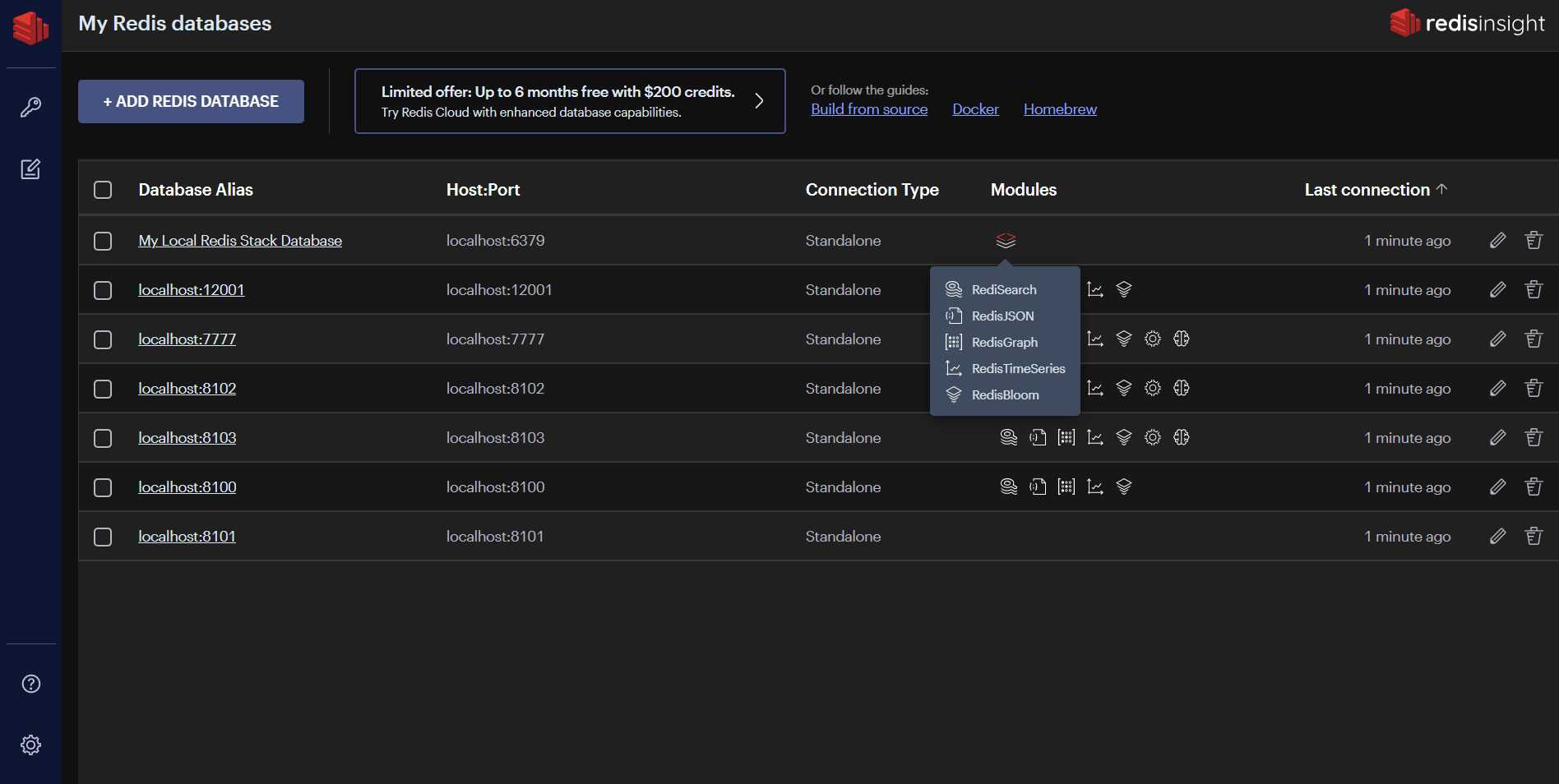
Browser

Browse, filter and visualize your key-value Redis data structures.

CRUD support for Lists, Hashes, Strings, Sets, Sorted Sets
CRUD support for RedisJSON
Group keys according to their namespaces

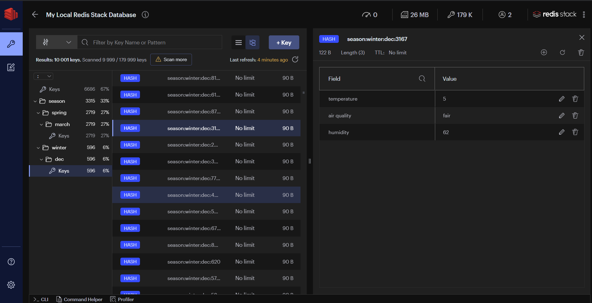
Profiler

Analyze every command sent to Redis in real time

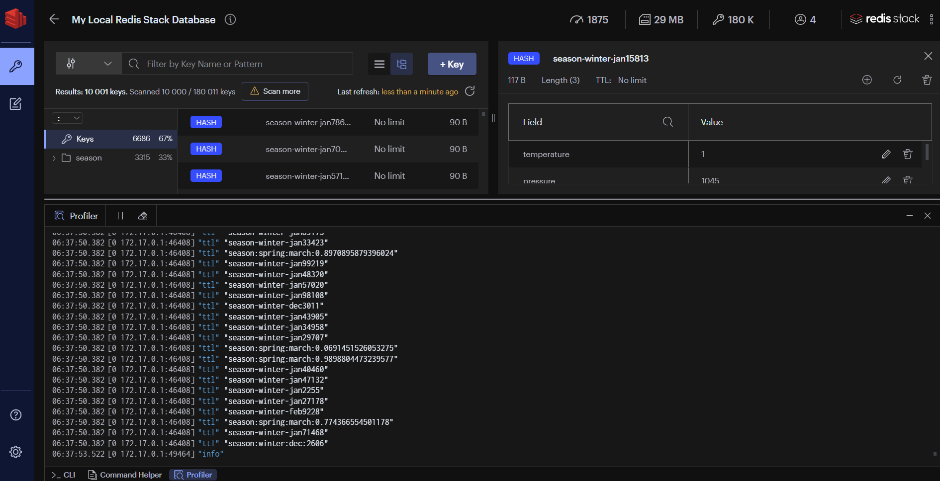
CLI

The CLI is accessible at any time within the applicaiton.

Employs integrated help to deliver intuitive assistance
Use together with a convenient command helper that lets you search and read on Redis commands.

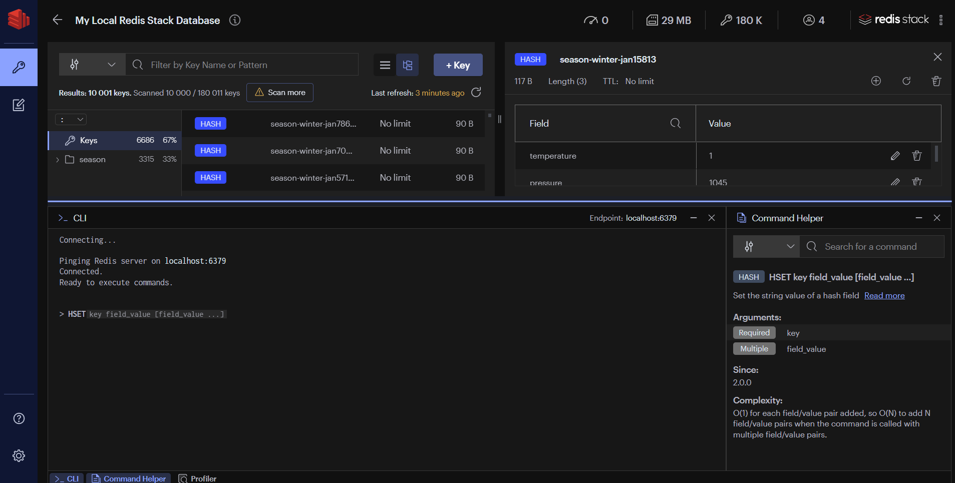
Workbench

Advanced command line interface with intelligent command auto-complete and complex data visualizations.

Built-in guides: you can conveniently discover Redis and Redis Stack capabilities using the built-in guides.
Command auto-complete support for all capabilities in Redis and Redis Stack.
Visualizations of your RediSearch index, queries, and aggregations
Visualizations of your RedisGraph and RedisTimeSeries data.

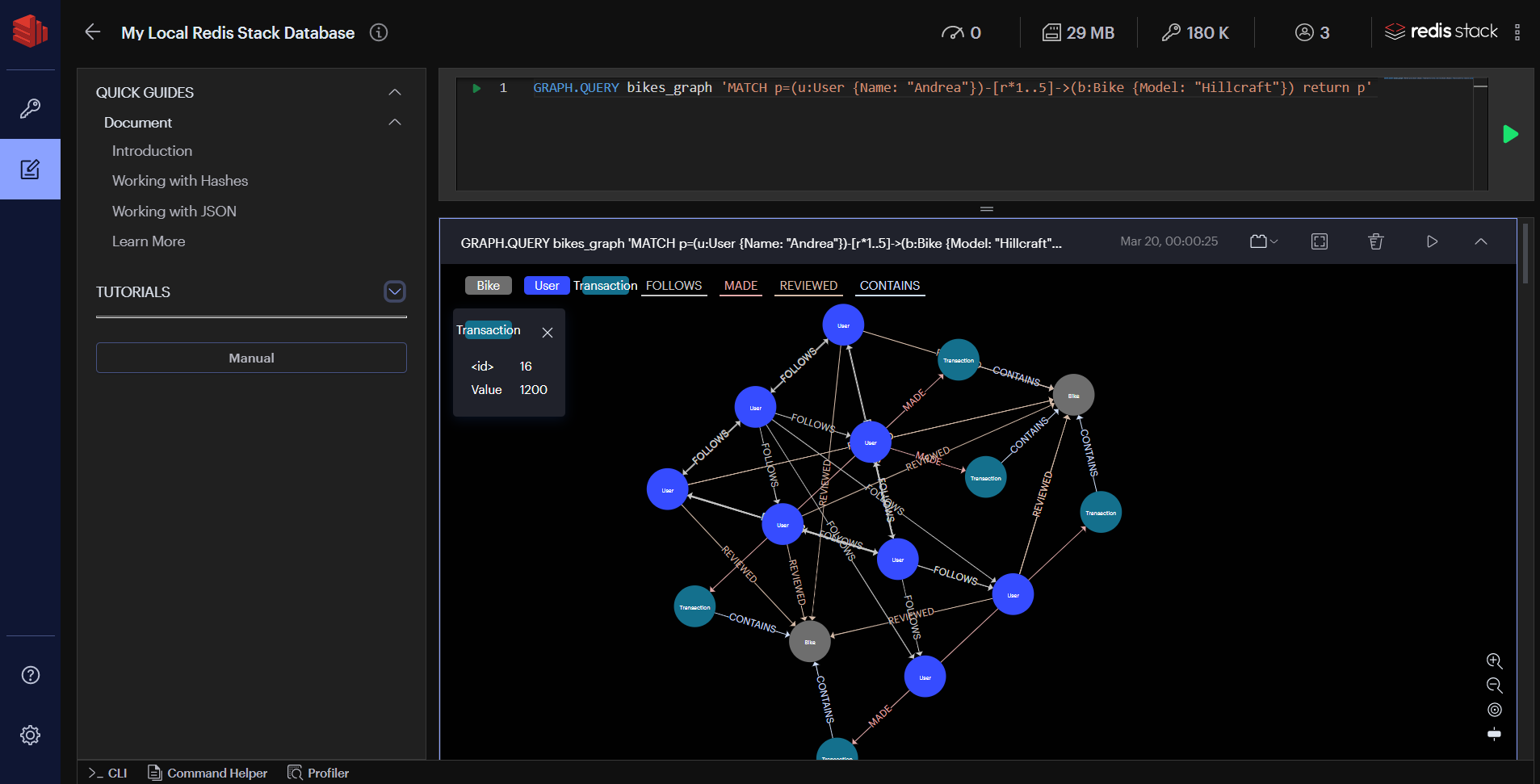
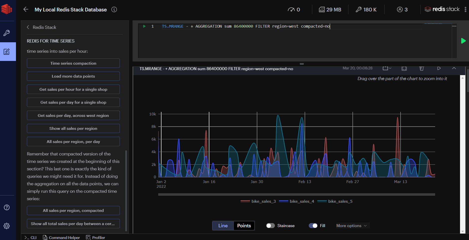
Plugins

With RedisInsight you can now also extend the core functionality by building your own data visualizations. See our plugin documentation for more information.

Telemetry

RedisInsight includes an opt-in telemetry system. This help us improve the developer experience of the app. We value your privacy; all collected data is anonymised.

Feedback

To provide your feedback, open a ticket in our RedisInsight repository.

License

RedisInsight is licensed under SSPL license.

3 - RediSearch

Queries, secondary indexing, and full-text search for Redis

RediSearch is a source available Redis module that provides queryability, secondary indexing, and full-text search for Redis.

Quick Links

Overview

RediSearch provides secondary indexing, full-text search, and a query language for Redis. These feature enable multi-field queries, aggregation, exact phrase matching, and numeric filtering for text queries.

Client libraries

Official and community client libraries are available for Python, Java, JavaScript, Ruby, Go, C#, and PHP.

See the clients page for the full list.

Cluster support

RediSearch provides a distributed cluster version that scales to billions of documents and hundreds of servers.

Commercial support

Commercial support for RediSearch is provided by Redis Ltd. See the Redis Ltd. website for more info and contact information.

Primary features

RediSearch supports the following features:

Secondary indexing
Multi-field queries
Aggregation
Full-text indexing of multiple fields in a documents
Incremental indexing without performance loss
Document ranking (provided manually by the user at index time)
Boolean queries with AND, OR, NOT operators between sub-queries
Optional query clauses
Prefix-based searches
Field weights
Auto-complete suggestions (with fuzzy prefix suggestions)
Exact-phrase search and slop-based search
Stemming-based query expansion for many languages (using Snowball)
Support for custom functions for query expansion and scoring (see Extensions)
Numeric filters and ranges
Geo-filtering using the Redis own geo commands
Unicode support (UTF-8 input required)
Retrieval of full document contents or only their ids
Document deletion and updating with index garbage collection
Partial and conditional document updates

Supported Platforms

RediSearch is developed and tested on Linux and macOS on x86_64 CPUs.

Atom CPUs are not supported.

References

Videos

Course

RU203: Querying, Indexing, and Full-Text Search - An online RediSearch course from Redis University.

Blog posts

Mailing List / Forum

Got questions? Feel free to ask at the RediSearch forum.

License

Redis Source Available License Agreement - see LICENSE

3.1 - Commands

Commands Overview

RediSearch API

Details on module's commands can be filtered for a specific module or command, e.g., FT. The details also include the syntax for the commands, where:

Command and subcommand names are in uppercase, for example FT.CREATE
Optional arguments are enclosed in square brackets, for example [NOCONTENT]
Additional optional arguments are indicated by three period characters, for example ...

The query commands, i.e. FT.SEARCH and FT.AGGREGATE, require an index name as their first argument, then a query, i.e. hello|world, and finally additional parameters or attributes.

See the quick start page on creating and indexing and start searching.

See the reference page for more details on the various parameters.

3.2 - Quick start

Quick start guide

Quick Start Guide for RediSearch

Redis Cloud

RediSearch is available on all Redis Cloud managed services. Redis Cloud Essentials offers a completely free managed database up to 30MB.

Get started here

Running with Docker

docker run -p 6379:6379 redislabs/redisearch:latest

Download and running binaries

First download the pre-compiled version from the Redis download center.

Next, run Redis with RediSearch:

$ redis-server --loadmodule /path/to/module/src/redisearch.so

Building and running from source

First, clone the git repo (make sure not to omit the --recursive option, to properly clone submodules):

git clone --recursive https://github.com/RediSearch/RediSearch.git
cd RediSearch

Next, install dependencies:

On macOS:

make setup

On Linux:

sudo make setup

Next, build:

make build

Finally, run Redis with RediSearch:

make run

For more elaborate build instructions, see the Development page.

Creating an index with fields and weights (default weight is 1.0)

127.0.0.1:6379> FT.CREATE myIdx ON HASH PREFIX 1 doc: SCHEMA title TEXT WEIGHT 5.0 body TEXT url TEXT
OK

Adding documents to the index

127.0.0.1:6379> hset doc:1 title "hello world" body "lorem ipsum" url "http://redis.io" 
(integer) 3

Searching the index

127.0.0.1:6379> FT.SEARCH myIdx "hello world" LIMIT 0 10
1) (integer) 1
2) "doc:1"
3) 1) "title"
   2) "hello world"
   3) "body"
   4) "lorem ipsum"
   5) "url"
   6) "http://redis.io"

!!! note Input is expected to be valid utf-8 or ASCII. The engine cannot handle wide character unicode at the moment.

Dropping the index

127.0.0.1:6379> FT.DROPINDEX myIdx 
OK

Adding and getting Auto-complete suggestions

127.0.0.1:6379> FT.SUGADD autocomplete "hello world" 100
OK

127.0.0.1:6379> FT.SUGGET autocomplete "he"
1) "hello world"

3.3 - Configuration

Details about configuration options

Run-time configuration

RediSearch supports a few run-time configuration options that should be determined when loading the module. In time more options will be added.

Passing Configuration Options During Loading

In general, passing configuration options is done by appending arguments after the --loadmodule argument in the command line, loadmodule configuration directive in a Redis config file, or the MODULE LOAD command. For example:

In redis.conf:

loadmodule redisearch.so OPT1 OPT2

From redis-cli:

127.0.0.6379> MODULE load redisearch.so OPT1 OPT2

From command line:

$ redis-server --loadmodule ./redisearch.so OPT1 OPT2

Setting Configuration Options At Run-Time

As of v1.4.1, the FT.CONFIG allows setting some options during runtime. In addition, the command can be used to view the current run-time configuration options.

RediSearch configuration options

TIMEOUT

The maximum amount of time in milliseconds that a search query is allowed to run. If this time is exceeded we return the top results accumulated so far, or an error depending on the policy set with ON_TIMEOUT. The timeout can be disabled by setting it to 0.

!!! note Timeout refers to query time only. Parsing the query is not counted towards timeout. If timeout was not reached during the search, finalizing operation such as loading documents' content or reducers, continue.

Default

500

Example

$ redis-server --loadmodule ./redisearch.so TIMEOUT 100

ON_TIMEOUT {policy}

The response policy for queries that exceed the TIMEOUT setting.

The policy can be one of the following:

RETURN: this policy will return the top results accumulated by the query until it timed out.
FAIL: will return an error when the query exceeds the timeout value.

Default

RETURN

Example

$ redis-server --loadmodule ./redisearch.so ON_TIMEOUT fail

SAFEMODE

!! Deprecated in v1.6. From this version, SAFEMODE is the default. If you still like to re-enable the concurrent mode for writes, use CONCURRENT_WRITE_MODE !!

If present in the argument list, RediSearch will turn off concurrency for query processing, and work in a single thread.

This is useful if data consistency is extremely important, and avoids a situation where deletion of documents while querying them can cause momentarily inconsistent results (i.e. documents that were valid during the invocation of the query are not returned because they were deleted during query processing).

Default

Off (not present)

Example

$ redis-server --loadmodule ./redisearch.so SAFEMODE

Notes

deprecated in v1.6

CONCURRENT_WRITE_MODE

If enabled, write queries will be performed concurrently. For now only the tokenization part is executed concurrently. The actual write operation still requires holding the Redis Global Lock.

Default

Not set - "disabled"

Example

$ redis-server --loadmodule ./redisearch.so CONCURRENT_WRITE_MODE

Notes

added in v1.6

EXTLOAD {file_name}

If present, we try to load a RediSearch extension dynamic library from the specified file path. See Extensions for details.

Default

None

Example

$ redis-server --loadmodule ./redisearch.so EXTLOAD ./ext/my_extension.so

MINPREFIX

The minimum number of characters we allow for prefix queries (e.g. hel*). Setting it to 1 can hurt performance.

Default

Example

$ redis-server --loadmodule ./redisearch.so MINPREFIX 3

MAXPREFIXEXPANSIONS

The maximum number of expansions we allow for query prefixes. Setting it too high can cause performance issues. If MAXPREFIXEXPANSIONS is reached, the query will continue with the first acquired results.

Default

200

Example

$ redis-server --loadmodule ./redisearch.so MAXPREFIXEXPANSIONS 1000

!!! Note "MAXPREFIXEXPANSIONS replaces the deprecated config word MAXEXPANSIONS."

RediSearch considers these two configurations as synonyms.  The synonym was added to be more descriptive.

MAXDOCTABLESIZE

The maximum size of the internal hash table used for storing the documents. Notice, this configuration doesn't limit the amount of documents that can be stored but only the hash table internal array max size. Decreasing this property can decrease the memory overhead in case the index holds a small amount of documents that are constantly updated.

Default

1000000

Example

$ redis-server --loadmodule ./redisearch.so MAXDOCTABLESIZE 3000000

MAXSEARCHRESULTS

The maximum number of results to be returned by FT.SEARCH command if LIMIT is used. Setting value to -1 will remove the limit.

Default

1000000

Example

$ redis-server --loadmodule ./redisearch.so MAXSEARCHRESULTS 3000000

MAXAGGREGATERESULTS

The maximum number of results to be returned by FT.AGGREGATE command if LIMIT is used. Setting value to -1 will remove the limit.

Default

unlimited

Example

$ redis-server --loadmodule ./redisearch.so MAXAGGREGATERESULTS 3000000

FRISOINI {file_name}

If present, we load the custom Chinese dictionary from the specified path. See Using custom dictionaries for more details.

Default

Not set

Example

$ redis-server --loadmodule ./redisearch.so FRISOINI /opt/dict/friso.ini

CURSOR_MAX_IDLE

The maximum idle time (in ms) that can be set to the cursor api.

Default

"300000"

Example

$ redis-server --loadmodule ./redisearch.so CURSOR_MAX_IDLE 500000

Notes

added in v1.6

PARTIAL_INDEXED_DOCS

Enable/disable Redis command filter. The filter optimizes partial updates of hashes and may avoid reindexing of the hash if changed fields are not part of schema.

Considerations

The Redis command filter will be executed upon each Redis Command. Though the filter is optimized, this will introduce a small increase in latency on all commands.
This configuration is therefore best used with partial indexed documents where the non- indexed fields are updated frequently.

Default

"0"

Example

$ redis-server --loadmodule ./redisearch.so PARTIAL_INDEXED_DOCS 1

Notes

added in v2.0.0

GC_SCANSIZE

The garbage collection bulk size of the internal gc used for cleaning up the indexes.

Default

100

Example

$ redis-server --loadmodule ./redisearch.so GC_SCANSIZE 10

GC_POLICY

The policy for the garbage collector (GC). Supported policies are:

FORK: uses a forked thread for garbage collection (v1.4.1 and above). This is the default GC policy since version 1.6.1 and is ideal for general purpose workloads.
LEGACY: Uses a synchronous, in-process fork. This is ideal for read-heavy and append-heavy workloads with very few updates/deletes

Default

"FORK"

Example

$ redis-server --loadmodule ./redisearch.so GC_POLICY LEGACY

Notes

When the GC_POLICY is FORK it can be combined with the options below.

NOGC

If set, we turn off Garbage Collection for all indexes. This is used mainly for debugging and testing, and should not be set by users.

Default

Not set

Example

$ redis-server --loadmodule ./redisearch.so NOGC

FORK_GC_RUN_INTERVAL

Interval (in seconds) between two consecutive fork GC runs.

Default

"30"

Example

$ redis-server --loadmodule ./redisearch.so GC_POLICY FORK FORK_GC_RUN_INTERVAL 60

Notes

only to be combined with GC_POLICY FORK

FORK_GC_RETRY_INTERVAL

Interval (in seconds) in which RediSearch will retry to run fork GC in case of a failure. Usually, a failure could happen when the redis fork api does not allow for more than one fork to be created at the same time.

Default

"5"

Example

$ redis-server --loadmodule ./redisearch.so GC_POLICY FORK FORK_GC_RETRY_INTERVAL 10

Notes

only to be combined with GC_POLICY FORK
added in v1.4.16

FORK_GC_CLEAN_THRESHOLD

The fork GC will only start to clean when the number of not cleaned documents is exceeding this threshold, otherwise it will skip this run. While the default value is 100, it's highly recommended to change it to a higher number.

Default

"100"

Example

$ redis-server --loadmodule ./redisearch.so GC_POLICY FORK FORK_GC_CLEAN_THRESHOLD 10000

Notes

only to be combined with GC_POLICY FORK
added in v1.4.16

UPGRADE_INDEX

This configuration is a special configuration introduced to upgrade indices from v1.x RediSearch versions, further referred to as 'legacy indices.' This configuration option needs to be given for each legacy index, followed by the index name and all valid option for the index description ( also referred to as the ON arguments for following hashes) as described on ft.create api. See Upgrade to 2.0 for more information.

Default

There is no default for index name, and the other arguments have the same defaults as on FT.CREATE api

Example

$ redis-server --loadmodule ./redisearch.so UPGRADE_INDEX idx PREFIX 1 tt LANGUAGE french LANGUAGE_FIELD MyLang SCORE 0.5 SCORE_FIELD MyScore PAYLOAD_FIELD MyPayload UPGRADE_INDEX idx1

Notes

If the RDB file does not contain a legacy index that's specified in the configuration, a warning message will be added to the log file and loading will continue.
If the RDB file contains a legacy index that wasn't specified in the configuration loading will fail and the server won't start.

OSS_GLOBAL_PASSWORD

Global oss cluster password that will be used to connect to other shards.

Default

Not set

Example

$ redis-server --loadmodule ./redisearch.so OSS_GLOBAL_PASSWORD password

Notes

only relevant when Coordinator is used
added in v2.0.3

DEFAULT_DIALECT

The default DIALECT to be used by FT.CREATE, FT.AGGREGATE, FT.EXPLAIN, FT.EXPLAINCLI, and FT.SPECLCHECK.

Default

"1"

Example

$ redis-server --loadmodule ./redisearch.so DEFAULT_DIALECT 2

Notes

DIALECT 2 is required for Vector Similarity Search
added in v2.4.3

3.4 - Developer notes

Notes on debugging, testing and documentation

Developing RediSearch

Developing RediSearch involves setting up the development environment (which can be either Linux-based or macOS-based), building RediSearch, running tests and benchmarks, and debugging both the RediSearch module and its tests.

Cloning the git repository

By invoking the following command, RediSearch module and its submodules are cloned:

git clone --recursive https://github.com/RediSearch/RediSearch.git

Working in an isolated environment

There are several reasons to develop in an isolated environment, like keeping your workstation clean, and developing for a different Linux distribution. The most general option for an isolated environment is a virtual machine (it's very easy to set one up using Vagrant). Docker is even a more agile, as it offers an almost instant solution:

search=$(docker run -d -it -v $PWD:/build debian:bullseye bash)
docker exec -it $search bash

Then, from within the container, cd /build and go on as usual.

In this mode, all installations remain in the scope of the Docker container. Upon exiting the container, you can either re-invoke it with the above docker exec or commit the state of the container to an image and re-invoke it on a later stage:

docker commit $search redisearch1
docker stop $search
search=$(docker run -d -it -v $PWD:/build rediseatch1 bash)
docker exec -it $search bash

You can replace debian:bullseye with your OS of choice, with the host OS being the best choice (so you can run the RediSearch binary on your host once it is built).

Installing prerequisites

To build and test RediSearch one needs to install several packages, depending on the underlying OS. Currently, we support the Ubuntu/Debian, CentOS, Fedora, and macOS.

First, enter RediSearch directory.

If you have gnu make installed, you can execute,

make setup

Alternatively, invoke the following:

./deps/readies/bin/getpy2
./system-setup.py

Note that system-setup.py will install various packages on your system using the native package manager and pip. It will invoke sudo on its own, prompting for permission.

If you prefer to avoid that, you can:

Review system-setup.py and install packages manually,
Use system-setup.py --nop to display installation commands without executing them,
Use an isolated environment like explained above,
Use a Python virtual environment, as Python installations are known to be sensitive when not used in isolation: python2 -m virtualenv venv; . ./venv/bin/activate

Installing Redis

As a rule of thumb, you're better off running the latest Redis version.

If your OS has a Redis 6.x package, you can install it using the OS package manager.

Otherwise, you can invoke ./deps/readies/bin/getredis.

Getting help

make help provides a quick summary of the development features:

make setup         # install prerequisited (CAUTION: THIS WILL MODIFY YOUR SYSTEM)
make fetch         # download and prepare dependant modules

make build         # compile and link
  COORD=1|oss|rlec   # build coordinator (1|oss: Open Source, rlec: Enterprise)
  STATIC=1           # build as static lib
  LITE=1             # build RediSearchLight
  VECSIM_MARCH=arch  # architecture for VecSim build
  DEBUG=1            # build for debugging
  NO_TESTS=1         # disable unit tests
  WHY=1              # explain CMake decisions (in /tmp/cmake-why)
  FORCE=1            # Force CMake rerun (default)
  CMAKE_ARGS=...     # extra arguments to CMake
  VG=1               # build for Valgrind
  SAN=type           # build with LLVM sanitizer (type=address|memory|leak|thread) 
  SLOW=1             # do not parallelize build (for diagnostics)
make parsers       # build parsers code
make clean         # remove build artifacts
  ALL=1              # remove entire artifacts directory

make run           # run redis with RediSearch
  GDB=1              # invoke using gdb

make test          # run all tests (via ctest)
  COORD=1|oss|rlec   # test coordinator
  TEST=regex         # run tests that match regex
  TESTDEBUG=1        # be very verbose (CTest-related)
  CTEST_ARG=...      # pass args to CTest
  CTEST_PARALLEL=n   # run tests in give parallelism
make pytest        # run python tests (tests/pytests)
  COORD=1|oss|rlec   # test coordinator
  TEST=name          # e.g. TEST=test:testSearch
  RLTEST_ARGS=...    # pass args to RLTest
  REJSON=1|0         # also load RedisJSON module
  REJSON_PATH=path   # use RedisJSON module at `path`
  EXT=1              # External (existing) environment
  GDB=1              # RLTest interactive debugging
  VG=1               # use Valgrind
  VG_LEAKS=0         # do not search leaks with Valgrind
  SAN=type           # use LLVM sanitizer (type=address|memory|leak|thread) 
  ONLY_STABLE=1      # skip unstable tests
make c_tests       # run C tests (from tests/ctests)
make cpp_tests     # run C++ tests (from tests/cpptests)
  TEST=name          # e.g. TEST=FGCTest.testRemoveLastBlock

make callgrind     # produce a call graph
  REDIS_ARGS="args"

make pack          # create installation packages
  COORD=rlec         # pack RLEC coordinator ('redisearch' package)
  LITE=1             # pack RediSearchLight ('redisearch-light' package)
make deploy        # copy packages to S3
make release       # release a version

make docs          # create documentation
make deploy-docs   # deploy documentation

make platform      # build for specified platform
  OSNICK=nick        # platform to build for (default: host platform)
  TEST=1             # run tests after build
  PACK=1             # create package
  ARTIFACTS=1        # copy artifacts to host

make box           # create container with volumen mapping into /search
  OSNICK=nick        # platform spec
make sanbox        # create container with CLang Sanitizer

Building from source

make build will build RediSearch.

make build COORD=oss will build OSS RediSearch Coordinator.

make build STATIC=1 will build as a static lib

Notes:

Binary files are placed under bin, according to platform and build variant.
RediSearch uses CMake as its build system. make build will invoke both CMake and the subsequent make command that's required to complete the build.

Use make clean to remove built artifacts. make clean ALL=1 will remove the entire bin subdirectory.

Diagnosing build process

make build will build in parallel by default.

For purposes of build diagnosis, make build SLOW=1 VERBOSE=1 can be used to examine compilation commands.

Running Redis with RediSearch

The following will run redis and load RediSearch module.

make run

You can open redis-cli in another terminal to interact with it.

Running tests

There are several sets of unit tests:

C tests, located in tests/ctests, run by make c_tests.
C++ tests (enabled by GTest), located in tests/cpptests, run by make cpp_tests.
Python tests (enabled by RLTest), located in tests/pytests, run by make pytest.

One can run all tests by invoking make test. A single test can be run using the TEST parameter, e.g. make test TEST=regex.

Debugging

To build for debugging (enabling symbolic information and disabling optimization), run make DEBUG=1. One can the use make run DEBUG=1 to invoke gdb. In addition to the usual way to set breakpoints in gdb, it is possible to use the BB macro to set a breakpoint inside RediSearch code. It will only have an effect when running under gdb.

Similarly, Python tests in a single-test mode, one can set a breakpoint by using the BB() function inside a test.

3.5 - Client Libraries

List of RediSearch client libraries

RediSearch has several client libraries, written by the module authors and community members - abstracting the API in different programming languages.

While it is possible and simple to use the raw Redis commands API, in most cases it's easier to just use a client library abstracting it.

Currently available Libraries

Language	Library	Author	License
Python	redis-py	Redis	BSD
Python	redis-om	Redis	BSD-3-Clause
Java	Jedis	Redis	MIT
Java (Jedis client library)	JRediSearch	Redis Inc	BSD
Java	redis-om-spring	Redis	BSD-3-Clause
Java (Lettuce client library)	LettuceMod	Redis Inc	Apache-2.0
Java	Spring LettuceMod	Redis Labs	Apache-2.0
Java	redis-modules-java	dengliming	Apache-2.0
Go	redisearch-go	Redis Inc	BSD
JavaScript	Redis-om	Redis	BSD-3-Clause
TypeScript	Node-Redis	Redis	MIT
TypeScript	redis-modules-sdk	Dani Tseitlin	BSD-3-Clause
C#	NRediSearch	Marc Gravell	MIT
C#	RediSearchClient	Tom Hanks	MIT
C#	Redis.OM	Redis	BSD-3-Clause
PHP	php-redisearch	MacFJA	MIT
PHP	redisearch-php (for RediSearch v1)	Ethan Hann	MIT
PHP	Redisearch (for RediSearch v2)	Front	MIT
Ruby on Rails	redi_search_rails	Dmitry Polyakovsky	MIT
Ruby	redisearch-rb	Victor Ruiz	MIT
Ruby	redi_search	Nick Pezza	MIT

Other available Libraries

Language	Library	Author	License	Stars	Comments
Rust	redisearch-api-rs	Redis Inc	BSD		API for Redis Modules written in Rust

3.6 - Administration Guide

Administration of the RediSearch module

3.6.1 - General Administration

General Administration of the RediSearch module

RediSearch Administration Guide

RediSearch doesn't require any configuration to work, but there are a few things worth noting when running RediSearch on top of Redis.

Persistence

RediSearch supports both RDB and AOF based persistence. For a pure RDB set-up, nothing special is needed beyond the standard Redis RDB configuration.

AOF Persistence

While RediSearch supports working with AOF based persistence, as of version 1.1.0 it does not support "classic AOF" mode, which uses AOF rewriting. Instead, it only supports AOF with RDB preamble mode. In this mode, rewriting the AOF log just creates an RDB file, which is appended to.

To enable AOF persistence with RediSearch, add the two following lines to your redis.conf:

appendonly yes
aof-use-rdb-preamble yes

Master/Slave Replication

RediSearch supports replication inherently, and using a master/slave set-up, you can use slaves for high availability. On top of that, slaves can be used for searching, to load-balance read traffic.

Cluster Support

RediSearch will not work correctly on a cluster. The enterprise version of RediSearch, which is commercially available from Redis Labs, does support a cluster set up and scales to hundreds of nodes, billions of documents and terabytes of data. See the Redis Labs Website for more details.

3.6.2 - Upgrade to 2.0

Details about upgrading to RediSearch 2.x from 1.x

Upgrade to 2.0 when running in Redis OSS

!!! note For enterprise upgrade please refer to the following link.

v2 of RediSearch re-architects the way indices are kept in sync with the data. Instead of using FT.ADD command to index documents, RediSearch 2.0 follows hashes that match the index description regardless of how those were inserted or changed on Redis (HSET, HINCR, HDEL). The index description will filter hashes on a prefix of the key, and allows you to construct fine-grained filters with the FILTER option. This description can be defined during index creation (FT.CREATE).

v1.x indices (further referred to as legacy indices) don't have such index description. That is why you will need to supply their descriptions when upgrading to v2. During the upgrade to v2, you should add the descriptions via the module's configuration so RediSearch 2.0 will be able to load these legacy indexes.

UPGRADE_INDEX configuration

The upgrade index configuration allows you to specify the legacy index to upgrade. It needs to specify the index name and all the on hash arguments that can be defined on FT.CREATE command (notice that only the index name is mandatory, the other arguments have default values which are the same as the default values on FT.CREATE command). So for example, if you have a legacy index called idx, in order for RediSearch 2.0 to load it, the following configuration needs to be added to the server on start time:

redis-server --loadmodule redisearch.so UPGRADE_INDEX idx

It is also possible to specify the prefixes to follow. For example, assuming all the documents indexed by idx starts with the prefix idx:, the following will upgrade the legacy index idx:

redis-server --loadmodule redisearch.so UPGRADE_INDEX idx PREFIX 1 idx:

Upgrade Limitations

The way that the upgrade process works behind the scenes is that it redefines the index with the on hash index description given in the configuration and then reindexes the data. This comes with some limitations:

If NOSAVE was used, then it's not possible to upgrade because the data for reindexing does not exist.
If you have multiple indices, you need to find the way for RediSearch to identify which hashes belong to which index. You can do it either with a prefix or a filter.
If you have hashes that are not indexed, you will need to find a way so that RediSearch will be able to identify only the hashes that need to be indexed. This can be done using a prefix or a filter.

3.7 - Reference

Reference

3.7.1 - Query syntax

Details of the query syntax

Search Query Syntax

We support a simple syntax for complex queries with the following rules:

Multi-word phrases simply a list of tokens, e.g. foo bar baz, and imply intersection (AND) of the terms.
Exact phrases are wrapped in quotes, e.g "hello world".
OR Unions (i.e word1 OR word2), are expressed with a pipe (|), e.g. hello|hallo|shalom|hola.
NOT negation (i.e. word1 NOT word2) of expressions or sub-queries. e.g. hello -world. As of version 0.19.3, purely negative queries (i.e. -foo or -@title:(foo|bar)) are supported.
Prefix matches (all terms starting with a prefix) are expressed with a *. For performance reasons, a minimum prefix length is enforced (2 by default, but is configurable)
A special "wildcard query" that returns all results in the index - * (cannot be combined with anything else).
Selection of specific fields using the syntax hello @field:world.
Numeric Range matches on numeric fields with the syntax @field:[{min} {max}].
Geo radius matches on geo fields with the syntax @field:[{lon} {lat} {radius} {m|km|mi|ft}]
Tag field filters with the syntax @field:{tag | tag | ...}. See the full documentation on [tag fields|/Tags].
Optional terms or clauses: foo ~bar means bar is optional but documents with bar in them will rank higher.
Fuzzy matching on terms (as of v1.2.0): %hello% means all terms with Levenshtein distance of 1 from it.
An expression in a query can be wrapped in parentheses to disambiguate, e.g. (hello|hella) (world|werld).
Query attributes can be applied to individual clauses, e.g. (foo bar) => { $weight: 2.0; $slop: 1; $inorder: false; }
Combinations of the above can be used together, e.g hello (world|foo) "bar baz" bbbb

Pure negative queries

As of version 0.19.3 it is possible to have a query consisting of just a negative expression, e.g. -hello or -(@title:(foo|bar)). The results will be all the documents NOT containing the query terms.

!!! warning Any complex expression can be negated this way, however, caution should be taken here: if a negative expression has little or no results, this is equivalent to traversing and ranking all the documents in the index, which can be slow and cause high CPU consumption.

Field modifiers

As of version 0.12 it is possible to specify field modifiers in the query and not just using the INFIELDS global keyword.

Per query expression or sub-expression, it is possible to specify which fields it matches, by prepending the expression with the @ symbol, the field name and a : (colon) symbol.

If a field modifier precedes multiple words or expressions, it applies only to the adjacent expression.

If a field modifier precedes an expression in parentheses, it applies only to the expression inside the parentheses. The expression should be valid for the specified field, otherwise it is skipped.

Multiple modifiers can be combined to create complex filtering on several fields. For example, if we have an index of car models, with a vehicle class, country of origin and engine type, we can search for SUVs made in Korea with hybrid or diesel engines - with the following query:

FT.SEARCH cars "@country:korea @engine:(diesel|hybrid) @class:suv"

Multiple modifiers can be applied to the same term or grouped terms. e.g.:

FT.SEARCH idx "@title|body:(hello world) @url|image:mydomain"

This will search for documents that have "hello" and "world" either in the body or the title, and the term "mydomain" in their url or image fields.

Numeric filters in query

If a field in the schema is defined as NUMERIC, it is possible to either use the FILTER argument in the Redis request or filter with it by specifying filtering rules in the query. The syntax is @field:[{min} {max}] - e.g. @price:[100 200].

A few notes on numeric predicates

It is possible to specify a numeric predicate as the entire query, whereas it is impossible to do it with the FILTER argument.
It is possible to intersect or union multiple numeric filters in the same query, be it for the same field or different ones.
-inf, inf and +inf are acceptable numbers in a range. Thus greater-than 100 is expressed as [(100 inf].
Numeric filters are inclusive. Exclusive min or max are expressed with ( prepended to the number, e.g. [(100 (200].
It is possible to negate a numeric filter by prepending a - sign to the filter, e.g. returning a result where price differs from 100 is expressed as: @title:foo -@price:[100 100].

Tag filters

RediSearch (starting with version 0.91) allows a special field type called "tag field", with simpler tokenization and encoding in the index. The values in these fields cannot be accessed by general field-less search, and can be used only with a special syntax:

@field:{ tag | tag | ...}

e.g.

@cities:{ New York | Los Angeles | Barcelona }

Tags can have multiple words or include other punctuation marks other than the field's separator (, by default). Punctuation marks in tags should be escaped with a backslash (\). It is also recommended (but not mandatory) to escape spaces; The reason is that if a multi-word tag includes stopwords, it will create a syntax error. So tags like "to be or not to be" should be escaped as "to\ be\ or\ not\ to\ be". For good measure, you can escape all spaces within tags.

Notice that multiple tags in the same clause create a union of documents containing either tags. To create an intersection of documents containing all tags, you should repeat the tag filter several times, e.g.:

# This will return all documents containing all three cities as tags:
@cities:{ New York } @cities:{Los Angeles} @cities:{ Barcelona }

# This will return all documents containing either city:
@cities:{ New York | Los Angeles | Barcelona }

Tag clauses can be combined into any sub-clause, used as negative expressions, optional expressions, etc.

Geo filters in query

As of version 0.21, it is possible to add geo radius queries directly into the query language with the syntax @field:[{lon} {lat} {radius} {m|km|mi|ft}]. This filters the result to a given radius from a lon,lat point, defined in meters, kilometers, miles or feet. See Redis' own GEORADIUS command for more details as it is used internally for that).

Radius filters can be added into the query just like numeric filters. For example, in a database of businesses, looking for Chinese restaurants near San Francisco (within a 5km radius) would be expressed as: chinese restaurant @location:[-122.41 37.77 5 km].

Vector Similarity search in query

It is possible to add vector similarity queries directly into the query language. The basic syntax is "*=>[ KNN {num|$num} @vector $query_vec ]" for running K nearest neighbors query on @vector field. It is also possilbe to run a Hybrid Query on filtered results.

A Hybrid query allows the user to specify a filter criteria that ALL results in a KNN query must satisfy. The filter criteria can only include fields with non-vector indexes (e.g. indexes created on scalar values such as TEXT, PHONETIC, NUMERIC, GEO, etc)

The General syntax is {some filter query}=>[ KNN {num|$num} @vector $query_vec]. For example:

@published_year:[2020 2021] - Only entities published between 2020 and 2021.
=> - Separates filter query from vector query.
[KNN {num|$num} @vector_field $query_vec] - Return num nearest neighbors entities where query_vec is similar to the vector stored in @vector_field.

As of version 2.4, we allow vector similarity to be used once in the query. For more information on vector smilarity syntax, see Vector Fields, "Querying vector fields" section.

Prefix matching

On index updating, we maintain a dictionary of all terms in the index. This can be used to match all terms starting with a given prefix. Selecting prefix matches is done by appending * to a prefix token. For example:

hel* world

Will be expanded to cover (hello|help|helm|...) world.

A few notes on prefix searches

As prefixes can be expanded into many many terms, use them with caution. There is no magic going on, the expansion will create a Union operation of all suffixes.
As a protective measure to avoid selecting too many terms, and block redis, which is single threaded, there are two limitations on prefix matching:

Prefixes are limited to 2 letters or more. You can change this number by using the MINPREFIX setting on the module command line.
Expansion is limited to 200 terms or less. You can change this number by using the MAXEXPANSIONS setting on the module command line.

Prefix matching fully supports Unicode and is case insensitive.
Currently, there is no sorting or bias based on suffix popularity, but this is on the near-term roadmap.

Fuzzy matching

As of v1.2.0, the dictionary of all terms in the index can also be used to perform Fuzzy Matching. Fuzzy matches are performed based on Levenshtein distance (LD). Fuzzy matching on a term is performed by surrounding the term with '%', for example:

%hello% world

Will perform fuzzy matching on 'hello' for all terms where LD is 1.

As of v1.4.0, the LD of the fuzzy match can be set by the number of '%' surrounding it, so that %%hello%% will perform fuzzy matching on 'hello' for all terms where LD is 2.

The maximal LD for fuzzy matching is 3.

Wildcard queries

As of version 1.1.0, we provide a special query to retrieve all the documents in an index. This is meant mostly for the aggregation engine. You can call it by specifying only a single star sign as the query string - i.e. FT.SEARCH myIndex *.

This cannot be combined with any other filters, field modifiers or anything inside the query. It is technically possible to use the deprecated FILTER and GEOFILTER request parameters outside the query string in conjunction with a wildcard, but this makes the wildcard meaningless and only hurts performance.

Query attributes

As of version 1.2.0, it is possible to apply specific query modifying attributes to specific clauses of the query.

The syntax is (foo bar) => { $attribute: value; $attribute:value; ...}, e.g:

(foo bar) => { $weight: 2.0; $slop: 1; $inorder: true; }
~(bar baz) => { $weight: 0.5; }

The supported attributes are:

$weight: determines the weight of the sub-query or token in the overall ranking on the result (default: 1.0).

$slop: determines the maximum allowed "slop" (space between terms) in the query clause (default: 0).
$inorder: whether or not the terms in a query clause must appear in the same order as in the query, usually set alongside with $slop (default: false).
$phonetic: whether or not to perform phonetic matching (default: true). Note: setting this attribute on for fields which were not creates as PHONETIC will produce an error.

A few query examples

Simple phrase query - hello AND world
```
  hello world
```
Exact phrase query - hello FOLLOWED BY world
```
  "hello world"
```
Union: documents containing either hello OR world
```
  hello|world
```
Not: documents containing hello but not world
```
  hello -world
```
Intersection of unions
```
  (hello|halo) (world|werld)
```
Negation of union
```
  hello -(world|werld)
```
Union inside phrase
```
  (barack|barrack) obama
```
Optional terms with higher priority to ones containing more matches:
```
  obama ~barack ~michelle
```
Exact phrase in one field, one word in another field:
```
  @title:"barack obama" @job:president
```

Combined AND, OR with field specifiers:

  @title:"hello world" @body:(foo bar) @category:(articles|biographies)

Prefix Queries:

  hello worl*

  hel* worl*

  hello -worl*

Numeric Filtering - products named "tv" with a price range of 200-500:
```
  @name:tv @price:[200 500]
```
Numeric Filtering - users with age greater than 18:
```
  @age:[(18 +inf]
```

Mapping common SQL predicates to RediSearch

SQL Condition	RediSearch Equivalent	Comments
WHERE x='foo' AND y='bar'	@x:foo @y:bar	for less ambiguity use (@x:foo) (@y:bar)
WHERE x='foo' AND y!='bar'	@x:foo -@y:bar
WHERE x='foo' OR y='bar'	(@x:foo)\|(@y:bar)
WHERE x IN ('foo', 'bar','hello world')	@x:(foo\|bar\|"hello world")	quotes mean exact phrase
WHERE y='foo' AND x NOT IN ('foo','bar')	@y:foo (-@x:foo) (-@x:bar)
WHERE x NOT IN ('foo','bar')	-@x:(foo\|bar)
WHERE num BETWEEN 10 AND 20	@num:[10 20]
WHERE num >= 10	@num:[10 +inf]
WHERE num > 10	@num:[(10 +inf]
WHERE num < 10	@num:[-inf (10]
WHERE num <= 10	@num:[-inf 10]
WHERE num < 10 OR num > 20	@num:[-inf (10] \| @num:[(20 +inf]
WHERE name LIKE 'john%'	@name:john*

Technical note

The query parser is built using the Lemon Parser Generator and a Ragel based lexer. You can see the grammar definition at the git repo.

3.7.2 - Stop-words

Stop-words support

Stop-Words

RediSearch has a pre-defined default list of stop-words. These are words that are usually so common that they do not add much information to search, but take up a lot of space and CPU time in the index.

When indexing, stop-words are discarded and not indexed. When searching, they are also ignored and treated as if they were not sent to the query processor. This is done when parsing the query.

At the moment, the default stop-word list applies to all full-text indexes in all languages and can be overridden manually at index creation time.

Default stop-word list

The following words are treated as stop-words by default:

 a,    is,    the,   an,   and,  are, as,  at,   be,   but,  by,   for,
 if,   in,    into,  it,   no,   not, of,  on,   or,   such, that, their,
 then, there, these, they, this, to,  was, will, with

Overriding the default stop-words

Stop-words for an index can be defined (or disabled completely) on index creation using the STOPWORDS argument in the [FT.CREATE command.

The format is STOPWORDS {number} {stopword} ... where number is the number of stopwords given. The STOPWORDS argument must come before the SCHEMA argument. For example:

FT.CREATE myIndex STOPWORDS 3 foo bar baz SCHEMA title TEXT body TEXT

Disabling stop-words completely

Disabling stopwords completely can be done by passing STOPWORDS 0 on FT.CREATE.

Avoiding stop-word detection in search queries

In rare use cases, where queries are very long and are guaranteed by the client application to not contain stopwords, it is possible to avoid checking for them when parsing the query. This saves some CPU time and is only worth it if the query has dozens or more terms in it. Using this without verifying that the query doesn't contain stop-words might result in empty queries.

3.7.3 - Aggregations

Details of FT.AGGREGATE. Grouping and projections and functions

RediSearch Aggregations

Aggregations are a way to process the results of a search query, group, sort and transform them - and extract analytic insights from them. Much like aggregation queries in other databases and search engines, they can be used to create analytics reports, or perform Faceted Search style queries.

For example, indexing a web-server's logs, we can create a report for unique users by hour, country or any other breakdown; or create different reports for errors, warnings, etc.

Core concepts

The basic idea of an aggregate query is this:

Perform a search query, filtering for records you wish to process.
Build a pipeline of operations that transform the results by zero or more steps of:
- Group and Reduce: grouping by fields in the results, and applying reducer functions on each group.
- Sort: sort the results based on one or more fields.
- Apply Transformations: Apply mathematical and string functions on fields in the pipeline, optionally creating new fields or replacing existing ones
- Limit: Limit the result, regardless of sorting the result.
- Filter: Filter the results (post-query) based on predicates relating to its values.

The pipeline is dynamic and re-entrant, and every operation can be repeated. For example, you can group by property X, sort the top 100 results by group size, then group by property Y and sort the results by some other property, then apply a transformation on the output.

Figure 1: Aggregation Pipeline Example

Aggregate request format

The aggregate request's syntax is defined as follows:

FT.AGGREGATE
  {index_name:string}
  {query_string:string}
  [VERBATIM]
  [LOAD {nargs:integer} {property:string} ...]
  [GROUPBY
    {nargs:integer} {property:string} ...
    REDUCE
      {FUNC:string}
      {nargs:integer} {arg:string} ...
      [AS {name:string}]
    ...
  ] ...
  [SORTBY
    {nargs:integer} {string} ...
    [MAX {num:integer}] ...
  ] ...
  [APPLY
    {EXPR:string}
    AS {name:string}
  ] ...
  [FILTER {EXPR:string}] ...
  [LIMIT {offset:integer} {num:integer} ] ...
  [PARAMS {nargs} {name} {value} ... ]

Parameters in detail

Parameters which may take a variable number of arguments are expressed in the form of param {nargs} {property_1... property_N}. The first argument to the parameter is the number of arguments following the parameter. This allows RediSearch to avoid a parsing ambiguity in case one of your arguments has the name of another parameter. For example, to sort by first name, last name, and country, one would specify SORTBY 6 firstName ASC lastName DESC country ASC.

index_name: The index the query is executed against.
query_string: The base filtering query that retrieves the documents. It follows the exact same syntax as the search query, including filters, unions, not, optional, etc.
LOAD {nargs} {property} …: Load document fields from the document HASH objects. This should be avoided as a general rule of thumb. Fields needed for aggregations should be stored as SORTABLE (and optionally UNF to avoid any normalization), where they are available to the aggregation pipeline with very low latency. LOAD hurts the performance of aggregate queries considerably since every processed record needs to execute the equivalent of HMGET against a redis key, which when executed over millions of keys, amounts to very high processing times. The document ID can be loaded using @__key.
GROUPBY {nargs} {property}: Group the results in the pipeline based on one or more properties. Each group should have at least one reducer (See below), a function that handles the group entries, either counting them or performing multiple aggregate operations (see below).
REDUCE {func} {nargs} {arg} … [AS {name}]: Reduce the matching results in each group into a single record, using a reduction function. For example, COUNT will count the number of records in the group. See the Reducers section below for more details on available reducers.
The reducers can have their own property names using the AS {name} optional argument. If a name is not given, the resulting name will be the name of the reduce function and the group properties. For example, if a name is not given to COUNT_DISTINCT by property @foo, the resulting name will be count_distinct(@foo).
SORTBY {nargs} {property} {ASC|DESC} [MAX {num}]: Sort the pipeline up until the point of SORTBY, using a list of properties. By default, sorting is ascending, but ASC or DESC can be added for each property. nargs is the number of sorting parameters, including ASC and DESC. for example: SORTBY 4 @foo ASC @bar DESC.
MAX is used to optimized sorting, by sorting only for the n-largest elements. Although it is not connected to LIMIT, you usually need just SORTBY … MAX for common queries.
APPLY {expr} AS {name}: Apply a 1-to-1 transformation on one or more properties, and either store the result as a new property down the pipeline, or replace any property using this transformation. expr is an expression that can be used to perform arithmetic operations on numeric properties, or functions that can be applied on properties depending on their types (see below), or any combination thereof. For example: APPLY "sqrt(@foo)/log(@bar) + 5" AS baz will evaluate this expression dynamically for each record in the pipeline and store the result as a new property called baz, that can be referenced by further APPLY / SORTBY / GROUPBY / REDUCE operations down the pipeline.
LIMIT {offset} {num}. Limit the number of results to return just num results starting at index offset (zero based). AS mentioned above, it is much more efficient to use SORTBY … MAX if you are interested in just limiting the output of a sort operation.
However, limit can be used to limit results without sorting, or for paging the n-largest results as determined by SORTBY MAX. For example, getting results 50-100 of the top 100 results is most efficiently expressed as SORTBY 1 @foo MAX 100 LIMIT 50 50. Removing the MAX from SORTBY will result in the pipeline sorting all the records and then paging over results 50-100.
FILTER {expr}. Filter the results using predicate expressions relating to values in each result. They are is applied post-query and relate to the current state of the pipeline. See FILTER Expressions below for full details.
PARAMS {nargs} {name} {value}. Define one or more value parameters. Each parameter has a name and a value. Parameters can be referenced in the query string by a $, followed by the parameter name, e.g., $user, and each such reference in the search query to a parameter name is substituted by the corresponding parameter value. For example, with parameter definition PARAMS 4 lon 29.69465 lat 34.95126, the expression @loc:[$lon $lat 10 km] would be evaluated to @loc:[29.69465 34.95126 10 km]. Parameters cannot be referenced in the query string where concrete values are not allowed, such as in field names, e.g., @loc

Quick example

Let's assume we have log of visits to our website, each record containing the following fields/properties:

url (text, sortable)
timestamp (numeric, sortable) - unix timestamp of visit entry.
country (tag, sortable)
user_id (text, sortable, not indexed)

Example 1: unique users by hour, ordered chronologically.

First of all, we want all records in the index, because why not. The first step is to determine the index name and the filtering query. A filter query of * means "get all records":

FT.AGGREGATE myIndex "*"

Now we want to group the results by hour. Since we have the visit times as unix timestamps in second resolution, we need to extract the hour component of the timestamp. So we first add an APPLY step, that strips the sub-hour information from the timestamp and stores is as a new property, hour:

FT.AGGREGATE myIndex "*"
  APPLY "@timestamp - (@timestamp % 3600)" AS hour

Now we want to group the results by hour, and count the distinct user ids in each hour. This is done by a GROUPBY/REDUCE step:

FT.AGGREGATE myIndex "*"
  APPLY "@timestamp - (@timestamp % 3600)" AS hour
  
  GROUPBY 1 @hour
  	REDUCE COUNT_DISTINCT 1 @user_id AS num_users

Now we'd like to sort the results by hour, ascending:

FT.AGGREGATE myIndex "*"
  APPLY "@timestamp - (@timestamp % 3600)" AS hour
  
  GROUPBY 1 @hour
  	REDUCE COUNT_DISTINCT 1 @user_id AS num_users
  	
  SORTBY 2 @hour ASC

And as a final step, we can format the hour as a human readable timestamp. This is done by calling the transformation function timefmt that formats unix timestamps. You can specify a format to be passed to the system's strftime function (see documentation), but not specifying one is equivalent to specifying %FT%TZ to strftime.

FT.AGGREGATE myIndex "*"
  APPLY "@timestamp - (@timestamp % 3600)" AS hour
  
  GROUPBY 1 @hour
  	REDUCE COUNT_DISTINCT 1 @user_id AS num_users
  	
  SORTBY 2 @hour ASC
  
  APPLY timefmt(@hour) AS hour

Example 2: Sort visits to a specific URL by day and country:

In this example we filter by the url, transform the timestamp to its day part, and group by the day and country, simply counting the number of visits per group. sorting by day ascending and country descending.

FT.AGGREGATE myIndex "@url:\"about.html\""
    APPLY "@timestamp - (@timestamp % 86400)" AS day
    GROUPBY 2 @day @country
    	REDUCE count 0 AS num_visits 
    SORTBY 4 @day ASC @country DESC

GROUPBY reducers

GROUPBY step work similarly to SQL GROUP BY clauses, and create groups of results based on one or more properties in each record. For each group, we return the "group keys", or the values common to all records in the group, by which they were grouped together - along with the results of zero or more REDUCE clauses.

Each GROUPBY step in the pipeline may be accompanied by zero or more REDUCE clauses. Reducers apply some accumulation function to each record in the group and reduce them into a single record representing the group. When we are finished processing all the records upstream of the GROUPBY step, each group emits its reduced record.

For example, the simplest reducer is COUNT, which simply counts the number of records in each group.

If multiple REDUCE clauses exist for a single GROUPBY step, each reducer works independently on each result and writes its final output once. Each reducer may have its own alias determined using the AS optional parameter. If AS is not specified, the alias is the reduce function and its parameters, e.g. count_distinct(foo,bar).

Supported GROUPBY reducers

COUNT

Format

REDUCE COUNT 0

Description

Count the number of records in each group

COUNT_DISTINCT

Format

REDUCE COUNT_DISTINCT 1 {property}

Description

Count the number of distinct values for property.

!!! note The reducer creates a hash-set per group, and hashes each record. This can be memory heavy if the groups are big.

COUNT_DISTINCTISH

Format

REDUCE COUNT_DISTINCTISH 1 {property}

Description

Same as COUNT_DISTINCT - but provide an approximation instead of an exact count, at the expense of less memory and CPU in big groups.

!!! note The reducer uses HyperLogLog counters per group, at ~3% error rate, and 1024 Bytes of constant space allocation per group. This means it is ideal for few huge groups and not ideal for many small groups. In the former case, it can be an order of magnitude faster and consume much less memory than COUNT_DISTINCT, but again, it does not fit every user case.

SUM

Format

REDUCE SUM 1 {property}

Description

Return the sum of all numeric values of a given property in a group. Non numeric values if the group are counted as 0.

MIN

Format

REDUCE MIN 1 {property}

Description

Return the minimal value of a property, whether it is a string, number or NULL.

MAX

Format

REDUCE MAX 1 {property}

Description

Return the maximal value of a property, whether it is a string, number or NULL.

AVG

Format

REDUCE AVG 1 {property}

Description

Return the average value of a numeric property. This is equivalent to reducing by sum and count, and later on applying the ratio of them as an APPLY step.

STDDEV

Format

REDUCE STDDEV 1 {property}

Description

Return the standard deviation of a numeric property in the group.

QUANTILE

Format

REDUCE QUANTILE 2 {property} {quantile}

Description

Return the value of a numeric property at a given quantile of the results. Quantile is expressed as a number between 0 and 1. For example, the median can be expressed as the quantile at 0.5, e.g. REDUCE QUANTILE 2 @foo 0.5 AS median .

If multiple quantiles are required, just repeat the QUANTILE reducer for each quantile. e.g. REDUCE QUANTILE 2 @foo 0.5 AS median REDUCE QUANTILE 2 @foo 0.99 AS p99

TOLIST

Format

REDUCE TOLIST 1 {property}

Description

Merge all distinct values of a given property into a single array.

FIRST_VALUE

Format

REDUCE FIRST_VALUE {nargs} {property} [BY {property} [ASC|DESC]]

Description

Return the first or top value of a given property in the group, optionally by comparing that or another property. For example, you can extract the name of the oldest user in the group:

REDUCE FIRST_VALUE 4 @name BY @age DESC

If no BY is specified, we return the first value we encounter in the group.

If you with to get the top or bottom value in the group sorted by the same value, you are better off using the MIN/MAX reducers, but the same effect will be achieved by doing REDUCE FIRST_VALUE 4 @foo BY @foo DESC.

RANDOM_SAMPLE

Format

REDUCE RANDOM_SAMPLE {nargs} {property} {sample_size}

Description

Perform a reservoir sampling of the group elements with a given size, and return an array of the sampled items with an even distribution.

APPLY expressions

APPLY performs a 1-to-1 transformation on one or more properties in each record. It either stores the result as a new property down the pipeline, or replaces any property using this transformation.

The transformations are expressed as a combination of arithmetic expressions and built in functions. Evaluating functions and expressions is recursively nested and can be composed without limit. For example: sqrt(log(foo) * floor(@bar/baz)) + (3^@qaz % 6) or simply @foo/@bar.

If an expression or a function is applied to values that do not match the expected types, no error is emitted but a NULL value is set as the result.

APPLY steps must have an explicit alias determined by the AS parameter.

Literals inside expressions

Numbers are expressed as integers or floating point numbers, i.e. 2, 3.141, -34, etc. inf and -inf are acceptable as well.
Strings are quoted with either single or double quotes. Single quotes are acceptable inside strings quoted with double quotes and vice versa. Punctuation marks can be escaped with backslashes. e.g. "foo's bar" ,'foo\'s bar', "foo \"bar\"" .
Any literal or sub expression can be wrapped in parentheses to resolve ambiguities of operator precedence.

Arithmetic operations

For numeric expressions and properties, we support addition (+), subtraction (-), multiplication (*), division (/), modulo (%) and power (^). We currently do not support bitwise logical operators.

Note that these operators apply only to numeric values and numeric sub expressions. Any attempt to multiply a string by a number, for instance, will result in a NULL output.

List of field APPLY functions

Function	Description	Example
exists(s)	Checks whether a field exists in a document.	`exists(@field)`

List of numeric APPLY functions

Function	Description	Example
log(x)	Return the logarithm of a number, property or sub-expression	`log(@foo)`
abs(x)	Return the absolute number of a numeric expression	`abs(@foo-@bar)`
ceil(x)	Round to the smallest value not less than x	`ceil(@foo/3.14)`
floor(x)	Round to largest value not greater than x	`floor(@foo/3.14)`
log2(x)	Return the logarithm of x to base 2	`log2(2^@foo)`
exp(x)	Return the exponent of x, i.e. `e^x`	`exp(@foo)`
sqrt(x)	Return the square root of x	`sqrt(@foo)`

List of string APPLY functions

Function
upper(s)	Return the uppercase conversion of s	`upper('hello world')`
lower(s)	Return the lowercase conversion of s	`lower("HELLO WORLD")`
startswith(s1,s2)	Return `1` if s2 is the prefix of s1, `0` otherwise.	`startswith(@field, "company")`
contains(s1,s2)	Return the number of occurrences of s2 in s1, `0` otherwise. If s2 is an empty string, return `length(s1) + 1`.	`contains(@field, "pa")`
substr(s, offset, count)	Return the substring of s, starting at offset and having count characters. If offset is negative, it represents the distance from the end of the string. If count is -1, it means "the rest of the string starting at offset".	`substr("hello", 0, 3)` `substr("hello", -2, -1)`
format( fmt, ...)	Use the arguments following `fmt` to format a string. Currently the only format argument supported is `%s` and it applies to all types of arguments.	`format("Hello, %s, you are %s years old", @name, @age)`
matched_terms([max_terms=100])	Return the query terms that matched for each record (up to 100), as a list. If a limit is specified, we will return the first N matches we find - based on query order.	`matched_terms()`
split(s, [sep=","], [strip=" "])	Split a string by any character in the string sep, and strip any characters in strip. If only s is specified, we split by commas and strip spaces. The output is an array.	split("foo,bar")

List of date/time APPLY functions

Function	Description
timefmt(x, [fmt])	Return a formatted time string based on a numeric timestamp value x. See strftime for formatting options. Not specifying `fmt` is equivalent to `%FT%TZ`.
parsetime(timesharing, [fmt])	The opposite of timefmt() - parse a time format using a given format string
day(timestamp)	Round a Unix timestamp to midnight (00:00) start of the current day.
hour(timestamp)	Round a Unix timestamp to the beginning of the current hour.
minute(timestamp)	Round a Unix timestamp to the beginning of the current minute.
month(timestamp)	Round a unix timestamp to the beginning of the current month.
dayofweek(timestamp)	Convert a Unix timestamp to the day number (Sunday = 0).
dayofmonth(timestamp)	Convert a Unix timestamp to the day of month number (1 .. 31).
dayofyear(timestamp)	Convert a Unix timestamp to the day of year number (0 .. 365).
year(timestamp)	Convert a Unix timestamp to the current year (e.g. 2018).
monthofyear(timestamp)	Convert a Unix timestamp to the current month (0 .. 11).

List of geo APPLY functions

Function	Description	Example
geodistance(field,field)	Return distance in meters.	`geodistance(@field1,@field2)`
geodistance(field,"lon,lat")	Return distance in meters.	`geodistance(@field,"1.2,-3.4")`
geodistance(field,lon,lat)	Return distance in meters.	`geodistance(@field,1.2,-3.4)`
geodistance("lon,lat",field)	Return distance in meters.	`geodistance("1.2,-3.4",@field)`
geodistance("lon,lat","lon,lat")	Return distance in meters.	`geodistance("1.2,-3.4","5.6,-7.8")`
geodistance("lon,lat",lon,lat)	Return distance in meters.	`geodistance("1.2,-3.4",5.6,-7.8)`
geodistance(lon,lat,field)	Return distance in meters.	`geodistance(1.2,-3.4,@field)`
geodistance(lon,lat,"lon,lat")	Return distance in meters.	`geodistance(1.2,-3.4,"5.6,-7.8")`
geodistance(lon,lat,lon,lat)	Return distance in meters.	`geodistance(1.2,-3.4,5.6,-7.8)`

FT.AGGREGATE myIdx "*"  LOAD 1 location  APPLY "geodistance(@location,\"-1.1,2.2\")" AS dist

To print out the distance:

FT.AGGREGATE myIdx "*"  LOAD 1 location  APPLY "geodistance(@location,\"-1.1,2.2\")" AS dist

Note: Geo field must be preloaded using LOAD.

Results can also be sorted by distance:

FT.AGGREGATE idx "*" LOAD 1 @location FILTER "exists(@location)" APPLY "geodistance(@location,-117.824722,33.68590)" AS dist SORTBY 2 @dist DESC

Note: Make sure no location is missing, otherwise the SORTBY will not return any result. Use FILTER to make sure you do the sorting on all valid locations.

FILTER expressions

FILTER expressions filter the results using predicates relating to values in the result set.

The FILTER expressions are evaluated post-query and relate to the current state of the pipeline. Thus they can be useful to prune the results based on group calculations. Note that the filters are not indexed and will not speed the processing per se.

Filter expressions follow the syntax of APPLY expressions, with the addition of the conditions ==, !=, <, <=, >, >=. Two or more predicates can be combined with logical AND (&&) and OR (||). A single predicate can be negated with a NOT prefix (!).

For example, filtering all results where the user name is 'foo' and the age is less than 20 is expressed as:

FT.AGGREGATE 
  ...
  FILTER "@name=='foo' && @age < 20"
  ...

Several filter steps can be added, although at the same stage in the pipeline, it is more efficient to combine several predicates into a single filter step.

Cursor API

FT.AGGREGATE ... WITHCURSOR [COUNT {read size} MAXIDLE {idle timeout}]
FT.CURSOR READ {idx} {cid} [COUNT {read size}]
FT.CURSOR DEL {idx} {cid}

You can use cursors with FT.AGGREGATE, with the WITHCURSOR keyword. Cursors allow you to consume only part of the response, allowing you to fetch additional results as needed. This is much quicker than using LIMIT with offset, since the query is executed only once, and its state is stored on the server.

To use cursors, specify the WITHCURSOR keyword in FT.AGGREGATE, e.g.

FT.AGGREGATE idx * WITHCURSOR

This will return a response of an array with two elements. The first element is the actual (partial) results, and the second is the cursor ID. The cursor ID can then be fed to FT.CURSOR READ repeatedly, until the cursor ID is 0, in which case all results have been returned.

To read from an existing cursor, use FT.CURSOR READ, e.g.

FT.CURSOR READ idx 342459320

Assuming 342459320 is the cursor ID returned from the FT.AGGREGATE request.

Here is an example in pseudo-code:

response, cursor = FT.AGGREGATE "idx" "redis" "WITHCURSOR";
while (1) {
  processResponse(response)
  if (!cursor) {
    break;
  }
  response, cursor = FT.CURSOR read "idx" cursor
}

Note that even if the cursor is 0, a partial result may still be returned.

Cursor settings

Read size

You can control how many rows are read per each cursor fetch by using the COUNT parameter. This parameter can be specified both in FT.AGGREGATE (immediately after WITHCURSOR) or in FT.CURSOR READ.

FT.AGGREGATE idx query WITHCURSOR COUNT 10

Will read 10 rows at a time.

You can override this setting by also specifying COUNT in CURSOR READ, e.g.

FT.CURSOR READ idx 342459320 COUNT 50

Will return at most 50 results.

The default read size is 1000

Timeouts and limits

Because cursors are stateful resources which occupy memory on the server, they have a limited lifetime. In order to safeguard against orphaned/stale cursors, cursors have an idle timeout value. If no activity occurs on the cursor before the idle timeout, the cursor is deleted. The idle timer resets to 0 whenever the cursor is read from using CURSOR READ.

The default idle timeout is 300000 milliseconds (or 300 seconds). You can modify the idle timeout using the MAXIDLE keyword when creating the cursor. Note that the value cannot exceed the default 300s.

FT.AGGREGATE idx query WITHCURSOR MAXIDLE 10000

Will set the limit for 10 seconds.

Other cursor commands

Cursors can be explicitly deleted using the CURSOR DEL command, e.g.

FT.CURSOR DEL idx 342459320

Note that cursors are automatically deleted if all their results have been returned, or if they have been timed out.

All idle cursors can be forcefully purged at once using FT.CURSOR GC idx 0 command. By default, RediSearch uses a lazy throttled approach to garbage collection, which collects idle cursors every 500 operations, or every second - whichever is later.

3.7.4 - Tokenization

Controlling Text Tokenization and Escaping

At the moment, RediSearch uses a very simple tokenizer for documents and a slightly more sophisticated tokenizer for queries. Both allow a degree of control over string escaping and tokenization.

Note: There is a different mechanism for tokenizing text and tag fields, this document refers only to text fields. For tag fields please refer to the Tag Fields documentation.

The rules of text field tokenization

All punctuation marks and whitespace (besides underscores) separate the document and queries into tokens. e.g. any character of ,.<>{}[]"':;!@#$%^&*()-+=~ will break the text into terms. So the text foo-bar.baz...bag will be tokenized into [foo, bar, baz, bag]
Escaping separators in both queries and documents is done by prepending a backslash to any separator. e.g. the text hello\-world hello-world will be tokenized as [hello-world, hello, world]. NOTE that in most languages you will need an extra backslash when formatting the document or query, to signify an actual backslash, so the actual text in redis-cli for example, will be entered as hello\\-world.
Underscores (_) are not used as separators in either document or query. So the text hello_world will remain as is after tokenization.
Repeating spaces or punctuation marks are stripped.
In Latin characters, everything gets converted to lowercase.
A backslash before the first digit will tokenize it as a term. This will translate - sign as NOT which otherwise will make the number negative. Add a backslash before . if you are searching for a float. (ex. -20 -> {-20} vs -\20 -> {NOT{20}})

3.7.5 - Sorting

Support for sorting query results

Sorting by Indexed Fields

As of RediSearch 0.15, it is possible to bypass the scoring function mechanism, and order search results by the value of different document properties (fields) directly - even if the sorting field is not used by the query. For example, you can search for first name and sort by last name.

Declaring Sortable Fields

When creating the index with FT.CREATE, you can declare TEXT and NUMERIC properties to be SORTABLE. When a property is sortable, we can later decide to order the results by its values. For example, in the following schema:

> FT.CREATE users SCHEMA first_name TEXT last_name TEXT SORTABLE age NUMERIC SORTABLE

The fields last_name and age are sortable, but first_name isn't. This means we can search by either first and/or last name, and sort by last name or age.

Note on sortable TEXT fields

In the current implementation, when declaring a sortable field, its content gets copied into a special location in the index, for fast access on sorting. This means that making long text fields sortable is very expensive, and you should be careful with it.

Normalization (UNF option)

By default, text fields get normalized and lowercased in a Unicode-safe way when stored for sorting. This means that America and america are considered equal in terms of sorting.

Using the argument UNF (un-normalized form) it is possible to disable the normalization and keep the original form of the value. Therefore, America will come before america.

Specifying SORTBY

If an index includes sortable fields, you can add the SORTBY parameter to the search request (outside the query body), and order the results by it. This overrides the scoring function mechanism, and the two cannot be combined. If WITHSCORES is specified along with SORTBY, the scores returned are simply the relative position of each result in the result set.

The syntax for SORTBY is:

SORTBY {field_name} [ASC|DESC]

field_name must be a sortable field defined in the schema.
ASC means the order will be ascending, DESC that it will be descending.
The default ordering is ASC if not specified otherwise.

Quick example

> FT.CREATE users SCHEMA first_name TEXT SORTABLE last_name TEXT age NUMERIC SORTABLE

# Add some users
> FT.ADD users user1 1.0 FIELDS first_name "alice" last_name "jones" age 35
> FT.ADD users user2 1.0 FIELDS first_name "bob" last_name "jones" age 36

# Searching while sorting

# Searching by last name and sorting by first name
> FT.SEARCH users "@last_name:jones" SORTBY first_name DESC

# Searching by both first and last name, and sorting by age
> FT.SEARCH users "alice jones" SORTBY age ASC

3.7.6 - Tags

Details about tag fields

Tag Fields

Tag fields are similar to full-text fields but use simpler tokenization and encoding in the index. The values in these fields cannot be accessed by general field-less search and can be used only with a special syntax.

The main differences between tag and full-text fields are:

We do not perform stemming on tag indexes.
The tokenization is simpler: The user can determine a separator (defaults to a comma) for multiple tags, and we only do whitespace trimming at the end of tags. Thus, tags can contain spaces, punctuation marks, accents, etc.
The only two transformations we perform are lower-casing (for latin languages only as of now) and whitespace trimming. Lower-case transformation can be disabled by passing CASESENSITIVE.
Tags cannot be found from a general full-text search. If a document has a field called "tags" with the values "foo" and "bar", searching for foo or bar without a special tag modifier (see below) will not return this document.
The index is much simpler and more compressed: We do not store frequencies, offset vectors of field flags. The index contains only document IDs encoded as deltas. This means that an entry in a tag index is usually one or two bytes long. This makes them very memory efficient and fast.
We can create up to 1024 tag fields per index.

Creating a tag field

Tag fields can be added to the schema in FT.ADD with the following syntax:

FT.CREATE ... SCHEMA ... {field_name} TAG [SEPARATOR {sep}] [CASESENSITIVE]

SEPARATOR defaults to a comma (,), and can be any printable ASCII character. For example:

CASESENSITIVE can be specified to keep the original letters case.

FT.CREATE idx ON HASH PREFIX 1 test: SCHEMA tags TAG SEPARATOR ";"

Querying tag fields

As mentioned above, just searching for a tag without any modifiers will not retrieve documents containing it.

The syntax for matching tags in a query is as follows (the curly braces are part of the syntax in this case):

   @<field_name>:{ <tag> | <tag> | ...}

For example, this query finds documents with either the tag hello world or foo bar:

    FT.SEARCH idx "@tags:{ hello world | foo bar }"

Tag clauses can be combined into any sub-clause, used as negative expressions, optional expressions, etc. For example, given the following index:

FT.CREATE idx ON HASH PREFIX 1 test: SCHEMA title TEXT price NUMERIC tags TAG SEPARATOR ";"

You can combine a full-text search on the title field, a numerical range on price, and match either the foo bar or hello world tag like this:

FT.SEARCH idx "@title:hello @price:[0 100] @tags:{ foo bar | hello world }

Tags support prefix matching with the regular * character:

FT.SEARCH idx "@tags:{ hell* }"
FT.SEARCH idx "@tags:{ hello\\ w* }"

Multiple tags in a single filter

Notice that including multiple tags in the same clause creates a union of all documents that contain any of the included tags. To create an intersection of documents containing all of the given tags, you should repeat the tag filter several times.

For example, imagine an index of travellers, with a tag field for the cities each traveller has visited:

FT.CREATE myIndex ON HASH PREFIX 1 traveller: SCHEMA name TEXT cities TAG

HSET traveller:1 name "John Doe" cities "New York, Barcelona, San Francisco"

For this index, the following query will return all the people who visited at least one of the following cities:

FT.SEARCH myIndex "@cities:{ New York | Los Angeles | Barcelona }"

But the next query will return all people who have visited all three cities:

FT.SEARCH myIndex "@cities:{ New York } @cities:{Los Angeles} @cities:{ Barcelona }"

Including punctuation in tags

A tag can include punctuation other than the field's separator (by default, a comma). You do not need to escape punctuation when using the HSET command to add the value to a Redis Hash.

For example, given the following index:

FT.CREATE punctuation ON HASH PREFIX 1 test: SCHEMA tags TAG

You can add tags that contain punctuation like this:

HSET test:1 tags "Andrew's Top 5,Justin's Top 5"

However, when you query for tags that contain punctuation, you must escape that punctuation with a backslash character (\).

NOTE: In most languages you will need an extra backslash. This is also the case in the redis-cli.

For example, querying for the tag Andrew's Top 5 in the redis-cli looks like this:

FT.SEARCH punctuation "@tags:{ Andrew\\'s Top 5 }"

Tags that contain multiple words

As the examples in this document show, a single tag can include multiple words. We recommend that you escape spaces when querying, though doing so is not required.

You escape spaces the same way that you escape punctuation -- by preceding the space with a backslash character (or two backslashes, depending on the programming language and environment).

Thus, you would escape the tag "to be or not to be" like so when querying in the redis-cli:

FT.SEARCH idx "@tags:{ to\\ be\\ or\\ not\\ to\\ be }"

You should escape spaces because if a tag includes multiple words and some of them are stop words like "to" or "be," a query that includes these words without escaping spaces will create a syntax error.

You can see what that looks like in the following example:

127.0.0.1:6379> FT.SEARCH idx "@tags:{ to be or not to be }"
(error) Syntax error at offset 27 near be

NOTE: Stop words are words that are so common that a search engine ignores them. We have a dedicated page about stop words in RediSearch if you would like to learn more.

Given the potential for syntax errors, we recommend that you escape all spaces within tag queries.

3.7.7 - Highlighting

Highlighting full-text results

Highlighting API

The highlighting API allows you to have only the relevant portions of document matching a search query returned as a result. This allows users to quickly see how a document relates to their query, with the search terms highlighted, usually in bold letters.

RediSearch implements high performance highlighting and summarization algorithms, with the following API:

Command syntax

FT.SEARCH ...
    SUMMARIZE [FIELDS {num} {field}] [FRAGS {numFrags}] [LEN {fragLen}] [SEPARATOR {sepstr}]
    HIGHLIGHT [FIELDS {num} {field}] [TAGS {openTag} {closeTag}]

There are two sub-commands commands used for highlighting. One is HIGHLIGHT which surrounds matching text with an open and/or close tag, and the other is SUMMARIZE which splits a field into contextual fragments surrounding the found terms. It is possible to summarize a field, highlight a field, or perform both actions in the same query.

Summarization

FT.SEARCH ...
    SUMMARIZE [FIELDS {num} {field}] [FRAGS {numFrags}] [LEN {fragLen}] [SEPARATOR {sepStr}]

Summarization will fragment the text into smaller sized snippets; each snippet will contain the found term(s) and some additional surrounding context.

RediSearch can perform summarization using the SUMMARIZE keyword. If no additional arguments are passed, all returned fields are summarized using built-in defaults.

The SUMMARIZE keyword accepts the following arguments:

FIELDS: If present, must be the first argument. This should be followed by the number of fields to summarize, which itself is followed by a list of fields. Each field present is summarized. If no FIELDS directive is passed, then all fields returned are summarized.
FRAGS: How many fragments should be returned. If not specified, a default of 3 is used.
LEN The number of context words each fragment should contain. Context words surround the found term. A higher value will return a larger block of text. If not specified, the default value is 20.
SEPARATOR The string used to divide between individual summary snippets. The default is ... which is common among search engines; but you may override this with any other string if you desire to programmatically divide them later on. You may use a newline sequence, as newlines are stripped from the result body anyway (thus, it will not be conflated with an embedded newline in the text)

Highlighting

FT.SEARCH ... HIGHLIGHT [FIELDS {num} {field}] [TAGS {openTag} {closeTag}]

Highlighting will highlight the found term (and its variants) with a user-defined tag. This may be used to display the matched text in a different typeface using a markup language, or to otherwise make the text appear differently.

RediSearch can perform highlighting using the HIGHLIGHT keyword. If no additional arguments are passed, all returned fields are highlighted using built-in defaults.

The HIGHLIGHT keyword accepts the following arguments:

FIELDS If present, must be the first argument. This should be followed by the number of fields to highlight, which itself is followed by a list of fields. Each field present is highlighted. If no FIELDS directive is passed, then all fields returned are highlighted.
TAGS If present, must be followed by two strings; the first is prepended to each term match, and the second is appended to it. If no TAGS are specified, a built-in tag value is appended and prepended.

Field selection

If no specific fields are passed to the RETURN, SUMMARIZE, or HIGHLIGHT keywords, then all of a document's fields are returned. However, if any of these keywords contain a FIELD directive, then the SEARCH command will only return the sum total of all fields enumerated in any of those directives.

The RETURN keyword is treated specially, as it overrides any fields specified in SUMMARIZE or HIGHLIGHT.

In the command RETURN 1 foo SUMMARIZE FIELDS 1 bar HIGHLIGHT FIELDS 1 baz, the fields foo is returned as-is, while bar and baz are not returned, because RETURN was specified, but did not include those fields.

In the command SUMMARIZE FIELDS 1 bar HIGHLIGHT FIELDS 1 baz, bar is returned summarized and baz is returned highlighted.

3.7.8 - Scoring

Full-text scoring functions

Scoring in RediSearch

RediSearch comes with a few very basic scoring functions to evaluate document relevance. They are all based on document scores and term frequency. This is regardless of the ability to use sortable fields. Scoring functions are specified by adding the SCORER {scorer_name} argument to a search query.

If you prefer a custom scoring function, it is possible to add more functions using the Extension API.

These are the pre-bundled scoring functions available in RediSearch and how they work. Each function is mentioned by registered name, that can be passed as a SCORER argument in FT.SEARCH.

TFIDF (default)

Basic TF-IDF scoring with a few extra features thrown inside:

For each term in each result, we calculate the TF-IDF score of that term to that document. Frequencies are weighted based on field weights that are pre-determined, and each term's frequency is normalized by the highest term frequency in each document.
We multiply the total TF-IDF for the query term by the a priory document score given on FT.ADD.
We give a penalty to each result based on "slop" or cumulative distance between the search terms: exact matches will get no penalty, but matches where the search terms are distant see their score reduced significantly. For each 2-gram of consecutive terms, we find the minimal distance between them. The penalty is the square root of the sum of the distances, squared - 1/sqrt(d(t2-t1)^2 + d(t3-t2)^2 + ...).

So for N terms in document D, T1...Tn, the resulting score could be described with this python function:

def get_score(terms, doc):
    # the sum of tf-idf
    score = 0

    # the distance penalty for all terms
    dist_penalty = 0

    for i, term in enumerate(terms):
        # tf normalized by maximum frequency
        tf = doc.freq(term) / doc.max_freq

        # idf is global for the index, and not calculated each time in real life
        idf = log2(1 + total_docs / docs_with_term(term))

        score += tf*idf

        # sum up the distance penalty
        if i > 0:
            dist_penalty += min_distance(term, terms[i-1])**2

    # multiply the score by the document score
    score *= doc.score

    # divide the score by the root of the cumulative distance
    if len(terms) > 1:
        score /= sqrt(dist_penalty)

    return score

TFIDF.DOCNORM

Identical to the default TFIDF scorer, with one important distinction:

Term frequencies are normalized by the length of the document (expressed as the total number of terms). The length is weighted, so that if a document contains two terms, one in a field that has a weight 1 and one in a field with a weight of 5, the total frequency is 6, not 2.

FT.SEARCH myIndex "foo" SCORER TFIDF.DOCNORM

BM25

A variation on the basic TF-IDF scorer, see this Wikipedia article for more info.

We also multiply the relevance score for each document by the a priory document score and apply a penalty based on slop as in TFIDF.

FT.SEARCH myIndex "foo" SCORER BM25

DISMAX

A simple scorer that sums up the frequencies of the matched terms; in the case of union clauses, it will give the maximum value of those matches. No other penalties or factors are applied.

It is not a 1 to 1 implementation of Solr's DISMAX algorithm but follows it in broad terms.

FT.SEARCH myIndex "foo" SCORER DISMAX

DOCSCORE

A scoring function that just returns the a priory score of the document without applying any calculations to it. Since document scores can be updated, this can be useful if you'd like to use an external score and nothing further.

FT.SEARCH myIndex "foo" SCORER DOCSCORE

HAMMING

Scoring by the (inverse) Hamming Distance between the documents' payload and the query payload. Since we are interested in the nearest neighbors, we inverse the hamming distance (1/(1+d)) so that a distance of 0 gives a perfect score of 1 and is the highest rank.

This works only if:

The document has a payload.
The query has a payload.
Both are exactly the same length.

Payloads are binary-safe, and having payloads with a length that's a multiple of 64 bits yields slightly faster results.

Example:

127.0.0.1:6379> FT.CREATE idx SCHEMA foo TEXT
OK
127.0.0.1:6379> FT.ADD idx 1 1 PAYLOAD "aaaabbbb" FIELDS foo hello
OK
127.0.0.1:6379> FT.ADD idx 2 1 PAYLOAD "aaaacccc" FIELDS foo bar
OK

127.0.0.1:6379> FT.SEARCH idx "*" PAYLOAD "aaaabbbc" SCORER HAMMING WITHSCORES
1) (integer) 2
2) "1"
3) "0.5" // hamming distance of 1 --> 1/(1+1) == 0.5
4) 1) "foo"
   2) "hello"
5) "2"
6) "0.25" // hamming distance of 3 --> 1/(1+3) == 0.25
7) 1) "foo"
   2) "bar"

3.7.9 - Extensions

Details about extensions for query expanders and scoring functions

Extending RediSearch

RediSearch supports an extension mechanism, much like Redis supports modules. The API is very minimal at the moment, and it does not yet support dynamic loading of extensions in run-time. Instead, extensions must be written in C (or a language that has an interface with C) and compiled into dynamic libraries that will be loaded at run-time.

There are two kinds of extension APIs at the moment:

Query Expanders, whose role is to expand query tokens (i.e. stemmers).
Scoring Functions, whose role is to rank search results in query time.

Registering and loading extensions

Extensions should be compiled into .so files, and loaded into RediSearch on initialization of the module.

Compiling
Extensions should be compiled and linked as dynamic libraries. An example Makefile for an extension can be found here.
That folder also contains an example extension that is used for testing and can be taken as a skeleton for implementing your own extension.
Loading
Loading an extension is done by appending EXTLOAD {path/to/ext.so} after the loadmodule configuration directive when loading RediSearch. For example:
```
$ redis-server --loadmodule ./redisearch.so EXTLOAD ./ext/my_extension.so
```
This causes RediSearch to automatically load the extension and register its expanders and scorers.

Initializing an extension

The entry point of an extension is a function with the signature:

int RS_ExtensionInit(RSExtensionCtx *ctx);

When loading the extension, RediSearch looks for this function and calls it. This function is responsible for registering and initializing the expanders and scorers.

It should return REDISEARCH_ERR on error or REDISEARCH_OK on success.

Example init function


#include <redisearch.h> //must be in the include path

int RS_ExtensionInit(RSExtensionCtx *ctx) {

  /* Register  a scoring function with an alias my_scorer and no special private data and free function */
  if (ctx->RegisterScoringFunction("my_scorer", MyCustomScorer, NULL, NULL) == REDISEARCH_ERR) {
    return REDISEARCH_ERR;
  }

  /* Register a query expander  */
  if (ctx->RegisterQueryExpander("my_expander", MyExpander, NULL, NULL) ==
      REDISEARCH_ERR) {
    return REDISEARCH_ERR;
  }

  return REDISEARCH_OK;
}

Calling your custom functions

When performing a query, you can tell RediSearch to use your scorers or expanders by specifying the SCORER or EXPANDER arguments, with the given alias. e.g.:

FT.SEARCH my_index "foo bar" EXPANDER my_expander SCORER my_scorer

NOTE: Expander and scorer aliases are case sensitive.

The query expander API

At the moment, we only support basic query expansion, one token at a time. An expander can decide to expand any given token with as many tokens it wishes, that will be Union-merged in query time.

The API for an expander is the following:

#include <redisearch.h> //must be in the include path

void MyQueryExpander(RSQueryExpanderCtx *ctx, RSToken *token) {
    ...
}

RSQueryExpanderCtx

RSQueryExpanderCtx is a context that contains private data of the extension, and a callback method to expand the query. It is defined as:

typedef struct RSQueryExpanderCtx {

  /* Opaque query object used internally by the engine, and should not be accessed */
  struct RSQuery *query;

  /* Opaque query node object used internally by the engine, and should not be accessed */
  struct RSQueryNode **currentNode;

  /* Private data of the extension, set on extension initialization */
  void *privdata;

  /* The language of the query, defaults to "english" */
  const char *language;

  /* ExpandToken allows the user to add an expansion of the token in the query, that will be
   * union-merged with the given token in query time. str is the expanded string, len is its length,
   * and flags is a 32 bit flag mask that can be used by the extension to set private information on
   * the token */
  void (*ExpandToken)(struct RSQueryExpanderCtx *ctx, const char *str, size_t len,
                      RSTokenFlags flags);

  /* SetPayload allows the query expander to set GLOBAL payload on the query (not unique per token)
   */
  void (*SetPayload)(struct RSQueryExpanderCtx *ctx, RSPayload payload);

} RSQueryExpanderCtx;

RSToken

RSToken represents a single query token to be expanded and is defined as:

/* A token in the query. The expanders receive query tokens and can expand the query with more query
 * tokens */
typedef struct {
  /* The token string - which may or may not be NULL terminated */
  const char *str;
  /* The token length */
  size_t len;
  
  /* 1 if the token is the result of query expansion */
  uint8_t expanded:1;

  /* Extension specific token flags that can be examined later by the scoring function */
  RSTokenFlags flags;
} RSToken;

The scoring function API

A scoring function receives each document being evaluated by the query, for final ranking. It has access to all the query terms that brought up the document,and to metadata about the document such as its a-priory score, length, etc.

Since the scoring function is evaluated per each document, potentially millions of times, and since redis is single threaded - it is important that it works as fast as possible and be heavily optimized.

A scoring function is applied to each potential result (per document) and is implemented with the following signature:

double MyScoringFunction(RSScoringFunctionCtx *ctx, RSIndexResult *res,
                                    RSDocumentMetadata *dmd, double minScore);

RSScoringFunctionCtx is a context that implements some helper methods.

RSIndexResult is the result information - containing the document id, frequency, terms, and offsets.

RSDocumentMetadata is an object holding global information about the document, such as its a-priory score.

minSocre is the minimal score that will yield a result that will be relevant to the search. It can be used to stop processing mid-way of before we even start.

The return value of the function is double representing the final score of the result. Returning 0 causes the result to be counted, but if there are results with a score greater than 0, they will appear above it. To completely filter out a result and not count it in the totals, the scorer should return the special value RS_SCORE_FILTEROUT (which is internally set to negative infinity, or -1/0).

RSScoringFunctionCtx

This is an object containing the following members:

*void privdata: a pointer to an object set by the extension on initialization time.
RSPayload payload: A Payload object set either by the query expander or the client.
int GetSlop(RSIndexResult *res): A callback method that yields the total minimal distance between the query terms. This can be used to prefer results where the "slop" is smaller and the terms are nearer to each other.

RSIndexResult

This is an object holding the information about the current result in the index, which is an aggregate of all the terms that resulted in the current document being considered a valid result.

See redisearch.h for details

RSDocumentMetadata

This is an object describing global information, unrelated to the current query, about the document being evaluated by the scoring function.

Example query expander

This example query expander expands each token with the term foo:

#include <redisearch.h> //must be in the include path

void DummyExpander(RSQueryExpanderCtx *ctx, RSToken *token) {
    ctx->ExpandToken(ctx, strdup("foo"), strlen("foo"), 0x1337);  
}

Example scoring function

This is an actual scoring function, calculating TF-IDF for the document, multiplying that by the document score, and dividing that by the slop:

#include <redisearch.h> //must be in the include path

double TFIDFScorer(RSScoringFunctionCtx *ctx, RSIndexResult *h, RSDocumentMetadata *dmd,
                   double minScore) {
  // no need to evaluate documents with score 0 
  if (dmd->score == 0) return 0;

  // calculate sum(tf-idf) for each term in the result
  double tfidf = 0;
  for (int i = 0; i < h->numRecords; i++) {
    // take the term frequency and multiply by the term IDF, add that to the total
    tfidf += (float)h->records[i].freq * (h->records[i].term ? h->records[i].term->idf : 0);
  }
  // normalize by the maximal frequency of any term in the document   
  tfidf /=  (double)dmd->maxFreq;

  // multiply by the document score (between 0 and 1)
  tfidf *= dmd->score;

  // no need to factor the slop if tfidf is already below minimal score
  if (tfidf < minScore) {
    return 0;
  }

  // get the slop and divide the result by it, making sure we prefer results with closer terms
  tfidf /= (double)ctx->GetSlop(h);
  
  return tfidf;
}

3.7.10 - Stemming

Stemming support

Stemming Support

RediSearch supports stemming - that is adding the base form of a word to the index. This allows the query for "going" to also return results for "go" and "gone", for example.

The current stemming support is based on the Snowball stemmer library, which supports most European languages, as well as Arabic and other. We hope to include more languages soon (if you need a specific language support, please open an issue).

For further details see the Snowball Stemmer website.

Supported languages

The following languages are supported and can be passed to the engine when indexing or querying, with lowercase letters:

arabic
armenian
danish
dutch
english
finnish
french
german
hungarian
italian
norwegian
portuguese
romanian
russian
serbian
spanish
swedish
tamil
turkish
yiddish
chinese (see below)

Chinese support

Indexing a Chinese document is different than indexing a document in most other languages because of how tokens are extracted. While most languages can have their tokens distinguished by separation characters and whitespace, this is not common in Chinese.

Chinese tokenization is done by scanning the input text and checking every character or sequence of characters against a dictionary of predefined terms and determining the most likely (based on the surrounding terms and characters) match.

RediSearch makes use of the Friso chinese tokenization library for this purpose. This is largely transparent to the user and often no additional configuration is required.

Using custom dictionaries

If you wish to use a custom dictionary, you can do so at the module level when loading the module. The FRISOINI setting can point to the location of a friso.ini file which contains the relevant settings and paths to the dictionary files.

Note that there is no "default" friso.ini file location. RedisSearch comes with its own friso.ini and dictionary files which are compiled into the module binary at build-time.

3.7.11 - Synonym

Synonym support

Synonyms Support

Overview

RediSearch supports synonyms - that is searching for synonyms words defined by the synonym data structure.

The synonym data structure is a set of groups, each group contains synonym terms. For example, the following synonym data structure contains three groups, each group contains three synonym terms:

{boy, child, baby}
{girl, child, baby}
{man, person, adult}

When these three groups are located inside the synonym data structure, it is possible to search for 'child' and receive documents contains 'boy', 'girl', 'child' and 'baby'.

The synonym search technique

We use a simple HashMap to map between the terms and the group ids. During building the index, we check if the current term appears in the synonym map, and if it does we take all the group ids that the term belongs to.

For each group id, we add another record to the inverted index called "~<id>" that contains the same information as the term itself. When performing a search, we check if the searched term appears in the synonym map, and if it does we take all the group ids the term is belong to. For each group id, we search for "~<id>" and return the combined results. This technique ensures that we return all the synonyms of a given term.

Handling concurrency

Since the indexing is performed in a separate thread, the synonyms map may change during the indexing, which in turn may cause data corruption or crashes during indexing/searches. To solve this issue, we create a read-only copy for indexing purposes. The read-only copy is maintained using ref count.

As long as the synonyms map does not change, the original synonym map holds a reference to its read-only copy so it will not be freed. Once the data inside the synonyms map has changed, the synonyms map decreses the reference count of its read only copy. This ensures that when all the indexers are done using the read only copy, then the read only copy will automatically freed. Also it ensures that the next time an indexer asks for a read-only copy, the synonyms map will create a new copy (contains the new data) and return it.

Quick example

# Create an index
> FT.CREATE idx schema t text

# Create a synonym group 
> FT.SYNUPDATE idx group1 hello world

# Insert documents
> HSET foo t hello
(integer) 1
> HSET bar t world
(integer) 1

# Search
> FT.SEARCH idx hello
1) (integer) 2
2) "foo"
3) 1) "t"
   2) "hello"
4) "bar"
5) 1) "t"
   2) "world"

3.7.12 - Payload

Payload support(deprecated)

Document Payloads

!!! note The payload feature is deprecated in 2.0

Usually, RediSearch stores documents as hash keys. But if you want to access some data for aggregation or scoring functions, we might want to store that data as an inline payload. This will allow us to evaluate properties of a document for scoring purposes at very low cost.

Since the scoring functions already have access to the DocumentMetaData, which contains document flags and score, We can add custom payloads that can be evaluated in run-time.

Payloads are NOT indexed and are not treated by the engine in any way. They are simply there for the purpose of evaluating them in query time, and optionally retrieving them. They can be JSON objects, strings, or preferably, if you are interested in fast evaluation, some sort of binary encoded data which is fast to decode.

Adding payloads for documents

When inserting a document using FT.ADD, you can ask RediSearch to store an arbitrary binary safe string as the document payload. This is done with the PAYLOAD keyword:

FT.ADD {index_name} {doc_id} {score} PAYLOAD {payload} FIELDS {field} {data}...

Evaluating payloads in query time

When implementing a scoring function, the signature of the function exposed is:

double (*ScoringFunction)(DocumentMetadata *dmd, IndexResult *h);

!!! note Currently, scoring functions cannot be dynamically added, and forking the engine and replacing them is required.

DocumentMetaData includes a few fields, one of them being the payload. It wraps a simple byte array with arbitrary length:

typedef struct  {
    char *data,
    uint32_t len;
} DocumentPayload;

If no payload was set to the document, it is simply NULL. If it is not, you can go ahead and decode it. It is recommended to encode some metadata about the payload inside it, like a leading version number, etc.

Retrieving payloads from documents

When searching, it is possible to request the document payloads from the engine.

This is done by adding the keyword WITHPAYLOADS to FT.SEARCH.

If WITHPAYLOADS is set, the payloads follow the document id in the returned result. If WITHSCORES is set as well, the payloads follow the scores. e.g.:

127.0.0.1:6379> FT.CREATE foo SCHEMA bar TEXT
OK
127.0.0.1:6379> FT.ADD foo doc2 1.0 PAYLOAD "hi there!" FIELDS bar "hello"
OK
127.0.0.1:6379> FT.SEARCH foo "hello" WITHPAYLOADS WITHSCORES
1) (integer) 1
2) "doc2"           # id
3) "1"              # score
4) "hi there!"      # payload
5) 1) "bar"         # fields
   2) "hello"

3.7.13 - Spellchecking

Query spelling correction support

Query Spelling Correction

Query spelling correction, a.k.a "did you mean", provides suggestions for misspelled search terms. For example, the term 'reids' may be a misspelled 'redis'.

In such cases and as of v1.4 RediSearch can be used for generating alternatives to misspelled query terms. A misspelled term is a full text term (i.e., a word) that is:

Not a stop word
Not in the index
At least 3 characters long

The alternatives for a misspelled term are generated from the corpus of already-indexed terms and, optionally, one or more custom dictionaries. Alternatives become spelling suggestions based on their respective Levenshtein distances (LD) from the misspelled term. Each spelling suggestion is given a normalized score based on its occurances in the index.

To obtain the spelling corrections for a query, refer to the documentation of the FT.SPELLCHECK command.

Custom dictionaries

A dictionary is a set of terms. Dictionaries can be added with terms, have terms deleted from them and have their entire contents dumped using the FT.DICTADD, FT.DICTDEL and FT.DICTDUMP commands, respectively.

Dictionaries can be used to modify the behavior of RediSearch's query spelling correction, by including or excluding their contents from potential spelling correction suggestions.

When used for term inclusion, the terms in a dictionary can be provided as spelling suggestions regardless their occurances (or lack of) in the index. Scores of suggestions from inclusion dictionaries are always 0.

Conversely, terms in an exlusion dictionary will never be returned as spelling alternatives.

3.7.14 - Phonetic

Phonetic matching

Phonetic Matching

Phonetic matching, a.k.a "Jon or John", allows searching for terms based on their pronunciation. This capability can be a useful tool when searching for names of people.

Phonetic matching is based on the use of a phonetic algorithm. A phonetic algorithm transforms the input term to an approximate representation of its pronunciation. This allows indexing terms, and consequently searching, by their pronunciation.

As of v1.4 RediSearch provides phonetic matching via the definition of text fields with the PHONETIC attribute. This causes the terms in such fields to be indexed both by their textual value as well as their phonetic approximation.

Performing a search on PHONETIC fields will, by default, also return results for phonetically similar terms. This behavior can be controlled with the $phonetic query attribute.

Phonetic algorithms support

RediSearch currently supports a single phonetic algorithm, the Double Metaphone (DM). It uses the implementation at slacy/double-metaphone, which provides general support for Latin languages.

3.7.15 - Vector similarity

Details about vector fields and vector similarity queries

Vector Fields

Vector fields offers the ability to use vector similarity queries in the FT.SEARCH command.

Vector Similarity search capability offers the ability to load, index and query vectors stored as fields in a redis hashes.

At present, the key functionalites offered are:

Realtime vector indexing supporting 2 Indexing Methods -
- FLAT - Brute-force index.
- HNSW - Modified version of nmslib/hnswlib which is the author's implementation of Efficient and robust approximate nearest neighbor search using Hierarchical Navigable Small World graphs.
Realtime vector update/delete - triggering update of the index.
K nearest neighbors queries supporting 3 distance metrics to measure the degree of similarity between vectors. Metrics:
- L2 - Euclidean distance between two vectors.
- IP - Internal product of two vectors.
- COSINE - Cosine similarity of two vectors.

Creating a vector field

Vector fields can be added to the schema in FT.CREATE with the following syntax:

FT.CREATE ... SCHEMA ... {field_name} VECTOR {algorithm} {count} [{attribute_name} {attribute_value} ...]

{algorithm}
Must be specified and be a supported vector similarity index algorithm. the supported algorithms are:
FLAT - brute force algorithm.
HNSW - Hierarchical Navigable Small World algorithm.
The algorithm attribute specify which algorithm to use when searching for the k most similar vectors in the index.
{count}
Specify the number of attributes for the index. Must be specified.
Notice that this attribute counts the total number of attributes passed for the index in the command, although algorithm parameters should be submitted as named arguments. For example:
```
FT.CREATE my_idx SCHEMA vec_field VECTOR FLAT 6 TYPE FLOAT32 DIM 128 DISTANCE_METRIC L2
```
Here we pass 3 parameters for the index (TYPE, DIM, DISTANCE_METRIC), and count counts the total number of attributes (6).
{attribute_name} {attribute_value}
Algorithm attributes for the creation of the vector index. Every algorithm has its own mandatory and optional attributes.

Specific creation attributes per algorithm

FLAT

Mandatory parameters
- TYPE - Vector type. Current supported type is FLOAT32.
- DIM - Vector dimention. should be positive integer.
- DISTANCE_METRIC - Supported distance metric. Currently one of {L2, IP, COSINE}
Optional parameters
- INITIAL_CAP - Initial vector capacity in the index. Effects memory allocation size of the index.
- BLOCK_SIZE - block size to hold BLOCK_SIZE amount of vectors in a contiguous array. This is useful when the index is dynamic with respect to addition and deletion. Defaults to 1048576 (1024*1024).

Example

FT.CREATE my_index1 
SCHEMA vector_field VECTOR 
FLAT 
10 
TYPE FLOAT32 
DIM 128 
DISTANCE_METRIC L2 
INITIAL_CAP 1000000 
BLOCK_SIZE 1000

HNSW

Mandatory parameters
- TYPE - Vector type. Current supported type is FLOAT32.
- DIM - Vector dimention. should be positive integer.
- DISTANCE_METRIC - Supported distance metric. Currently one of {L2, IP, COSINE}
Optional parameters
- INITIAL_CAP - Initial vector capacity in the index. Effects memory allocation size of the index.
- M - Number the maximal allowed outgoing edges for each node in the graph in each layer. on layer zero the maximal number of outgoing edges will be 2M. Defaults to 16.
- EF_CONSTRUCTION - Number the maximal allowed potential outgoing edges candidates for each node in the graph, during the graph building. Defaults to 200.
- EF_RUNTIME - The number of maximum top candidates to hold during the KNN search. Higher values of EF_RUNTIME will lead to a more accurate results on the expense of a longer runtime. Defaults to 10.

Example

FT.CREATE my_index2 
SCHEMA vector_field VECTOR 
HNSW 
14 
TYPE FLOAT32 
DIM 128 
DISTANCE_METRIC L2 
INITIAL_CAP 1000000 
M 40 
EF_CONSTRUCTION 250 
EF_RUNTIME 20

Querying vector fields

We allow using vector similarity queries in the FT.SEARCH "query" parameter. The syntax for vector similarity queries is *=>[{vector similarity query}] for running the query on an entire vector field, or {primary filter query}=>[{vector similarity query}] for running similarity query on the result of the primary filter query. To use a vector similarity query, you must specify the option DIALECT 2 in the command itself, or by setting the DEFAULT_DIALECT option to 2, either with the commandFT.CONFIG SET or when loading the redisearch module and passing it the argument DEFAULT_DIALECT 2.

As of version 2.4, we allow vector similarity to be used once in the query, and over the entire query filter.

Invalid example: "(@title:Matrix)=>[KNN 10 @v $B] @year:[2020 2022]"
Valid example: "(@title:Matrix @year:[2020 2022])=>[KNN 10 @v $B]"

The {vector similarity query} part inside the square brackets needs to be in the following format:

KNN { number | $number_attribute } @{vector field} $blob_attribute [{vector query param name} {value|$value_attribute} [...]] [ AS {score field name | $score_field_name_attribute}]

Every "*_attribute" parameter should refer to an attribute in the PARAMS section.

{ number | $number_attribute } - The number of requested results ("K").
@{vector field} - vector field should be a name of a vector field in the index.
$blob_attribute - An attribute that holds the query vector as blob. must be passed through the PARAMS section.
[{vector query param name} {value|$value_attribute} [...]] - An optional part for passing vector similarity query parameters. Parameters should come in key-value pairs and should be valid parameters for the query. see what runtime parameters are valid for each algorithm.
[ AS {score field name | $score_field_name_attribute}] - An optional part for specifying a score field name, for later sorting by the similarity score. By default the score field name is "__{vector field}_score" and it can be used for sorting without using AS {score field name} in the query.

Specific runtime attributes per algorithm

FLAT

Currently there are no runtime parameters available for FLAT indexes

HNSW

Optional parameters
- EF_RUNTIME - The number of maximum top candidates to hold during the KNN search. Higher values of EF_RUNTIME will lead to a more accurate results on the expense of a longer runtime. Defaults to the EF_RUNTIME value passed on creation (which defaults to 10).

A few notes

Although specifing K requested results, the default LIMIT in RediSearch is 10, so for getting all the returned results, make sure to specify LIMIT 0 {K} in your command.
By default, the resluts are sorted by their documents default RediSearch score. for getting the results sorted by similarity score, use SORTBY {score field name} as explained earlier.

Examples for querying vector fields

FT.SEARCH idx "*=>[KNN 100 @vec $BLOB]" PARAMS 2 BLOB "\12\a9\f5\6c" DIALECT 2

FT.SEARCH idx "*=>[KNN 100 @vec $BLOB]" PARAMS 2 BLOB "\12\a9\f5\6c" SORTBY __vec_score DIALECT 2

FT.SEARCH idx "*=>[KNN $K @vec $BLOB EF_RUNTIME $EF]" PARAMS 6 BLOB "\12\a9\f5\6c" K 10 EF 150 DIALECT 2

FT.SEARCH idx "*=>[KNN $K @vec $BLOB AS my_scores]" PARAMS 4 BLOB "\12\a9\f5\6c" K 10 SORTBY my_scores DIALECT 2

FT.SEARCH idx "(@title:Dune @num:[2020 2022])=>[KNN $K @vec $BLOB AS my_scores]" PARAMS 4 BLOB "\12\a9\f5\6c" K 10 SORTBY my_scores DIALECT 2

FT.SEARCH idx "(@type:{shirt} ~@color:{blue})=>[KNN $K @vec $BLOB AS my_scores]" PARAMS 4 BLOB "\12\a9\f5\6c" K 10 SORTBY my_scores DIALECT 2

3.8 - Design Documents

Design Documents details

3.8.1 - Internal design

Details about design choices and implementations

RediSearch internal design

RediSearch implements inverted indexes on top of Redis, but unlike previous implementations of Redis inverted indexes, it uses custom data encoding, that allows more memory and CPU efficient searches, and more advanced search features.

This document details some of the design choices and how these features are implemented.

Intro: Redis String DMA

The main feature that this module takes advantage of, is Redis Modules Strings DMA, or Direct Memory Access.

This feature is simple yet very powerful. It basically allows modules to allocate data on Redis string keys,then get a direct pointer to the data allocated by this key, without copying or serializing it.

This allows very fast access to huge amounts of memory, and since from the module's perspective, the string value is exposed simply as char *, it can be cast to any data structure.

You simply call RedisModule_StringTruncate to resize a memory chunk to the size needed, and RedisModule_StringDMA to get direct access to the memory in that key. See https://github.com/RedisLabs/RedisModulesSDK/blob/master/FUNCTIONS.md#redismodule_stringdma

We use this API in the module mainly to encode inverted indexes, and for other auxiliary data structures besides that.

A generic "Buffer" implementation using DMA strings can be found in redis_buffer.c. It automatically resizes the Redis string it uses as raw memory when the capacity needs to grow.

Inverted index encoding

An Inverted Index is the data structure at the heart of all search engines. The idea is simple - per each word or search term, we save a list of all the documents it appears in, and other data, such as term frequency, the offsets where the term appeared in the document, and more. Offsets are used for "exact match" type searches, or for ranking of results.

When a search is performed, we need to either traverse such an index, or intersect or union two or more indexes. Classic Redis implementations of search engines use sorted sets as inverted indexes. This works but has significant memory overhead, and also does not allow for encoding of offsets, as explained above.

RediSearch uses String DMA (see above) to efficiently encode inverted indexes. It combines Delta Encoding and Varint Encoding to encode entries, minimizing space used for indexes, while keeping decompression and traversal efficient.

For each "hit" (document/word entry), we encode:

The document Id as a delta from the previous document.
The term frequency, factored by the document's rank (see below)
Flags, that can be used to filter only specific fields or other user-defined properties.
An Offset Vector, of all the document offsets of the word.

!!! note Document ids as entered by the user are converted to internal incremental document ids, that allow delta encoding to be efficient, and let the inverted indexes be sorted by document id.

This allows for a single index hit entry to be encoded in as little as 6 bytes (Note that this is the best case. depending on the number of occurrences of the word in the document, this can get much higher).

To optimize searches, we keep two additional auxiliary data structures in different DMA string keys:

Skip Index: We keep a table of the index offset of 1/50 of the index entries. This allows faster lookup when intersecting inverted indexes, as not the entire list must be traversed.
Score Index: In simple single-word searches, there is no real need to traverse all the results, just the top N results the user is interested in. So we keep an auxiliary index of the top 20 or so entries for each term and use them when applicable.

Document and result ranking

Each document entered to the engine using FT.ADD, has a user assigned rank, between 0 and 1.0. This is used in combination with TF-IDF scoring of each word, to rank the results.

As an optimization, each inverted index hit is encoded with TF*Document_rank as its score, and only IDF is applied during searches. This may change in the future.

On top of that, in the case of intersection queries, we take the minimal distance between the terms in the query, and factor that into the ranking. The closest the terms are to each other, the better the result.

When searching, we keep a priority queue of the top N results requested, and eventually return them, sorted by rank.

Index Specs and field weights

When creating an "index" using FT.CREATE, the user specifies the fields to be indexed, and their respective weights. This can be used to give some document fields, like a title, more weight in ranking results.

For example:

FT.CREATE my_index title 10.0 body 1.0 url 2.0

Will create an index on fields named title, body and url, with scores of 10, 1 and 2 respectively.

When documents are indexed, the weights are taken from the saved Index Spec, that is stored in a special redis key, and only fields that are specified in this spec are indexed.

Document data storage

It is not mandatory to save the document data when indexing a document (specifying NOSAVE for FT.ADD will cause the document to be indexed but not saved).

If the user does save the document, we simply create a HASH key in Redis, containing all fields (including ones not indexed), and upon search, we simply perform an HGETALL query on each retrieved document, returning its entire data.

TODO: Document snippets should be implemented down the road,

Query Execution Engine

We use a chained-iterator based approach to query execution, similar to Python generators in concept.

We simply chain iterators that yield index hits. Those can be:

Read Iterators, reading hits one by one from an inverted index. i.e. hello
Intersect Iterators, aggregating two or more iterators, yielding only their intersection points. i.e. hello AND world
Exact Intersect Iterators - same as above, but yielding results only if the intersection is an exact phrase. i.e. hello NEAR world
Union Iterators - combining two or more iterators, and yielding a union of their hits. i.e. hello OR world

These are combined based on the query as an execution plan that is evaluated lazily. For example:

hello ==> read("hello")

hello world ==> intersect( read("hello"), read("world") )

"hello world" ==> exact_intersect( read("hello"), read("world") )

"hello world" foo ==> intersect(
                            exact_intersect(
                                read("hello"),
                                read("world")
                            ),
                            read("foo")
                      )

All these iterators are lazy evaluated, entry by entry, with constant memory overhead.

The "root" iterator is read by the query execution engine, and filtered for the top N results in it.

Numeric Filters

We support defining a field in the index schema as "NUMERIC", meaning you will be able to limit search results only to ones where the given value falls within a specific range. Filtering is done by adding FILTER predicates (more than one is supported) to your query. e.g.:

FT.SEARCH products "hd tv" FILTER price 100 (300

The filter syntax follows the ZRANGEBYSCORE semantics of Redis, meaning -inf and +inf are supported, and prepending ( to a number means an exclusive range.

As of release 0.6, the implementation uses a multi-level range tree, saving ranges at multiple resolutions, to allow efficient range scanning. Adding numeric filters can accelerate slow queries if the numeric range is small relative to the entire span of the filtered field. For example, a filter on dates focusing on a few days out of years of data, can speed a heavy query by an order of magnitude.

Auto-Complete and Fuzzy Suggestions

Another important feature for RediSearch is its auto-complete or suggest commands. It allows you to create dictionaries of weighted terms, and then query them for completion suggestions to a given user prefix. For example, if we put the term “lcd tv” into a dictionary, sending the prefix “lc” will return it as a result. The dictionary is modeled as a compressed trie (prefix tree) with weights, that is traversed to find the top suffixes of a prefix.

RediSearch also allows for Fuzzy Suggestions, meaning you can get suggestions to user prefixes even if the user has a typo in the prefix. This is enabled using a Levenshtein Automaton, allowing efficient searching of the dictionary for all terms within a maximal Levenshtein distance of a term or prefix. Then suggested are weighted based on both their original score and distance from the prefix typed by the user. Currently we support (for performance reasons) only suggestions where the prefix is up to 1 Levenshtein distance away from the typed prefix.

However, since searching for fuzzy prefixes, especially very short ones, will traverse an enormous amount of suggestions (in fact, fuzzy suggestions for any single letter will traverse the entire dictionary!), it is recommended to use this feature carefully, and only when considering the performance penalty it incurs. Since Redis is single threaded, blocking it for any amount of time means no other queries can be processed at that time.

To support unicode fuzzy matching, we use 16-bit "runes" inside the trie and not bytes. This increases memory consumption if the text is purely ASCII, but allows completion with the same level of support to all modern languages. This is done in the following manner:

We assume all input to FT.SUG* commands is valid utf-8.
We convert the input strings to 32-bit Unicode, optionally normalizing, case-folding and removing accents on the way. If the conversion fails it's because the input is not valid utf-8.
We trim the 32-bit runes to 16-bit runes using the lower 16 bits. These can be used for insertion, deletion, and search.
We convert the output of searches back to utf-8.

3.8.2 - Technical overview

Technical details of the internal design of indexing and querying with RediSearch

RediSearch Technical Overview

Abstract

RediSearch is a powerful text search and secondary indexing engine, built on top of Redis as a Redis Module.

Unlike other Redis search libraries, it does not use the internal data structures of Redis like sorted sets. Using its own highly optimized data structures and algorithms, it allows for advanced search features, high performance, and low memory footprint. It can perform simple text searches, as well as complex structured queries, filtering by numeric properties and geographical distances.

RediSearch supports continuous indexing with no performance degradation, maintaining concurrent loads of querying and indexing. This makes it ideal for searching frequently updated databases, without the need for batch indexing and service interrupts.

RediSearch's Enterprise version supports scaling the search engine across many servers, allowing it to easily grow to billions of documents on hundreds of servers.

All of this is done while taking advantage of Redis' robust architecture and infrastructure. Utilizing Redis' protocol, replication, persistence, clustering - RediSearch delivers a powerful yet simple to manage and maintain search and indexing engine, that can be used as a standalone database, or to augment existing Redis databases with advanced powerful indexing capabilities.

Main features

Full-Text indexing of multiple fields in a document, including:
- Exact phrase matching.
- Stemming in many languages.
- Chinese tokenization support.
- Prefix queries.
- Optional, negative and union queries.
Distributed search on billions of documents.
Numeric property indexing.
Geographical indexing and radius filters.
Incremental indexing without performance loss.
A structured query language for advanced queries:
- Unions and intersections
- Optional and negative queries
- Tag filtering
- Prefix matching
A powerful auto-complete engine with fuzzy matching.
Multiple scoring models and sorting by values.
Concurrent low-latency insertion and updates of documents.
Concurrent searches allowing long-running queries without blocking Redis.
An extension mechanism allowing custom scoring models and query extension.
Support for indexing existing Hash objects in Redis databases.

Indexing documents

In order to search effectively, RediSearch needs to know how to index documents. A document may have several fields, each with its own weight (e.g. a title is usually more important than the text itself. The engine can also use numeric or geographical fields for filtering. Hence, the first step is to create the index definition, which tells RediSearch how to treat the documents we will add. For example, to define an index of products, indexing their title, description, brand, and price, the index creation would look like:

FT.CREATE my_index SCHEMA 
    title TEXT WEIGHT 5
    description TEXT 
    brand TEXT 
    PRICE numeric

When we will add a document to this index, for example:

FT.ADD my_index doc1 1.0 FIELDS
    title "Acme 42 inch LCD TV"
    description "42 inch brand new Full-HD tv with smart tv capabilities"
    brand "Acme"
    price 300

This tells RediSearch to take the document, break each field into its terms ("tokenization") and index it, by marking the index for each of the terms in the index as contained in this document. Thus, the product is added immediately to the index and can now be found in future searches

Searching

Now that we have added products to our index, searching is very simple:

FT.SEARCH products "full hd tv"

This will tell RediSearch to intersect the lists of documents for each term and return all documents containing the three terms. Of course, more complex queries can be performed, and the full syntax of the query language is detailed below.

Data structures

RediSearch uses its own custom data structures and uses Redis' native structures only for storing the actual document content (using Hash objects).

Using specialized data structures allows faster searches and more memory effective storage of index records, utilizing compression techniques like delta encoding.

These are the data structures RediSearch uses under the hood:

Index and document metadata

For each search index, there is a root data structure containing the schema, statistics, etc - but most importantly, little compact metadata about each document indexed.

Internally, inside the index, RediSearch uses delta encoded lists of numeric, incremental, 32-bit document ids. This means that the user given keys or ids for documents, need to be replaced with the internal ids on indexing, and back to the original ids on search.

For that, RediSearch saves two tables, mapping the two kinds of ids in two ways (one table uses a compact trie, the other is simply an array where the internal document ID is the array index). On top of that, for each document, we store its user given a priory score, some status bits, and an optional "payload" attached to the document by the user.

Accessing the document metadata table is an order of magnitude faster than accessing the hash object where the document is actually saved, so scoring functions that need to access metadata about the document can operate fast enough.

Inverted index

For each term appearing in at least one document, we keep an inverted index, basically a list of all the documents where this term appears. The list is compressed using delta coding, and the document ids are always incrementing.

When the user indexes the documents "foo", "bar" and "baz" for example, they are assigned incrementing ids, For example 1025, 1045, 1080. When encoding them into the index, we only encode the first ID, followed by the deltas between each entry and the previous one, in this case, 1025, 20, 35.

Using variable-width encoding, we can use one byte to express numbers under 255, two bytes for numbers between 256 and 16383 and so on. This can compress the index by up to 75%.

On top of the ids, we save the frequency of each term in each document, a bit mask representing the fields in which the term appeared in the document, and a list of the positions in which the term appeared.

The structure of the default search record is as follows. Usually, all the entries are one byte long:

+----------------+------------+------------------+-------------+------------------------+
|  docId_delta   |  frequency | field mask       | offsets len | offset, offset, ....   |
|  (1-4 bytes)   | (1-2 bytes)| (1-16 bytes)     |  (1-2 bytes)| (1-2 bytes per offset) |
+----------------+------------+------------------+-------------+------------------------+

Optionally, we can choose not to save any one of those attributes besides the ID, degrading the features available to the engine.

Numeric index

Numeric properties are indexed in a special data structure that enables filtering by numeric ranges in an efficient way. One could view a numeric value as a term operating just like an inverted index. For example, all the products with the price $100 are in a specific list, that is intersected with the rest of the query (see Query Execution Engine).

However, in order to filer by a range of prices, we would have to intersect the query with all the distinct prices within that range - or perform a union query. If the range has many values in it, this becomes highly inefficient.

To avoid that, we group numeric entries with close values together, in a single "range node". These nodes are stored in binary range tree, that allows the engine to select the relevant nodes and union them together. Each entry in a range node contains a document Id, and the actual numeric value for that document. To further optimize, the tree uses an adaptive algorithm to try to merge as many nodes as possible within the same range node.

Tag index

Tag indexes are similar to full-text indexes, but use simpler tokenization and encoding in the index. The values in these fields cannot be accessed by general field-less search and can be used only with a special syntax.

The main differences between tag fields and full-text fields are:

The tokenization is simpler: The user can determine a separator (defaults to a comma) for multiple tags, and we only do whitespace trimming at the end of tags. Thus, tags can contain spaces, punctuation marks, accents, etc. The only two transformations we perform are lower-casing (for latin languages only as of now), and whitespace trimming.
Tags cannot be found from a general full-text search. If a document has a field called "tags" with the values "foo" and "bar", searching for foo or bar without a special tag modifier (see below) will not return this document.
The index is much simpler and more compressed: we only store document ids in the index, usually resulting in 1-2 bytes per index entry.

Geo index

Geo indexes utilize Redis' own geo-indexing capabilities. In query time, the geographical part of the query (a radius filter) is sent to Redis, returning only the ids of documents that are within that radius. Longitude and latitude should be passed as one string lon,lat. For example, 1.23,4.56.

Auto-complete

The auto-complete engine (see below for a fuller description) utilizes a compact trie or prefix tree, to encode terms and search them by prefix.

Query language

We support a simple syntax for complex queries, that can be combined together to express complex filtering and matching rules. The query is combined as a text string in the FT.SEARCH request and is parsed using a complex query parser.

Multi-word phrases simply a list of tokens, e.g. foo bar baz, and imply intersection (AND) of the terms.
Exact phrases are wrapped in quotes, e.g "hello world".
OR Unions (i.e word1 OR word2), are expressed with a pipe (|), e.g. hello|hallo|shalom|hola.
NOT negation (i.e. word1 NOT word2) of expressions or sub-queries. e.g. hello -world.
Prefix matches (all terms starting with a prefix) are expressed with a * following a 2-letter or longer prefix.
Selection of specific fields using the syntax @field:hello world.
Numeric Range matches on numeric fields with the syntax @field:[{min} {max}].
Geo radius matches on geo fields with the syntax @field:[{lon} {lat} {radius} {m|km|mi|ft}]
Tag field filters with the syntax @field:{tag | tag | ...}. See the full documentation on tag fields.
Optional terms or clauses: foo ~bar means bar is optional but documents with bar in them will rank higher.

Complex queries example

Expressions can be combined together to express complex rules. For example, let's assume we have a database of products, where each entity has the fields title, brand, tags and price.

Expressing a generic search would be simply:

lcd tv

This would return documents containing these terms in any field. Limiting the search to specific fields (title only in this case) is expressed as:

@title:(lcd tv)

Numeric filters can be combined to filter price within a price range:

    @title:(lcd tv) 
    @price:[100 500.2]

Multiple text fields can be accessed in different query clauses, for example, to select products of multiple brands:

    @title:(lcd tv)
    @brand:(sony | samsung | lg)
    @price:[100 500.2]

Tag fields can be used to index multi-term properties without actual full-text tokenization:

    @title:(lcd tv) 
    @brand:(sony | samsung | lg) 
    @tags:{42 inch | smart tv} 
    @price:[100 500.2]

And negative clauses can also be added, in this example to filter out plasma and CRT TVs:

    @title:(lcd tv) 
    @brand:(sony | samsung | lg) 
    @tags:{42 inch | smart tv} 
    @price:[100 500.2]

    -@tags:{plasma | crt}

Scoring model

RediSearch comes with a few very basic scoring functions to evaluate document relevance. They are all based on document scores and term frequency. This is regardless of the ability to use sortable fields (see below). Scoring functions are specified by adding the SCORER {scorer_name} argument to a search request.

If you prefer a custom scoring function, it is possible to add more functions using the Extension API.

These are the pre-bundled scoring functions available in RediSearch:

TFIDF (Default)
Basic TF-IDF scoring with document score and proximity boosting factored in.
TFIDF.DOCNORM Identical to the default TFIDF scorer, with one important distinction:
BM25
A variation on the basic TF-IDF scorer, see this Wikipedia article for more info.
DISMAX
A simple scorer that sums up the frequencies of the matched terms; in the case of union clauses, it will give the maximum value of those matches.
DOCSCORE
A scoring function that just returns the priory score of the document without applying any calculations to it. Since document scores can be updated, this can be useful if you'd like to use an external score and nothing further.

Sortable fields

It is possible to bypass the scoring function mechanism, and order search results by the value of different document properties (fields) directly - even if the sorting field is not used by the query. For example, you can search for first name and sort by the last name.

When creating the index with FT.CREATE, you can declare TEXT and NUMERIC properties to be SORTABLE. When a property is sortable, we can later decide to order the results by its values. For example, in the following schema:

> FT.CREATE users SCHEMA first_name TEXT last_name TEXT SORTABLE age NUMERIC SORTABLE

Would allow the following query:

FT.SEARCH users "john lennon" SORTBY age DESC

Result highlighting and summarisation

Highlighting allows users to only the relevant portions of document matching a search query returned as a result. This allows users to quickly see how a document relates to their query, with the search terms highlighted, usually in bold letters.

RediSearch implements high performance highlighting and summarization algorithms, with the following API:

FT.SEARCH ...
    SUMMARIZE [FIELDS {num} {field}] [FRAGS {numFrags}] [LEN {fragLen}] [SEPARATOR {separator}]
    HIGHLIGHT [FIELDS {num} {field}] [TAGS {openTag} {closeTag}]

Summarisation will fragment the text into smaller sized snippets; each snippet will contain the found term(s) and some additional surrounding context.

Auto-completion

Another important feature for RediSearch is its auto-complete engine. This allows users to create dictionaries of weighted terms, and then query them for completion suggestions to a given user prefix. Completions can have "payloads" - a user-provided piece of data that can be used for display. For example, completing the names of users, it is possible to add extra metadata about users to be displayed al

For example, if a user starts to put the term “lcd tv” into a dictionary, sending the prefix “lc” will return the full term as a result. The dictionary is modeled as a compact trie (prefix tree) with weights, which is traversed to find the top suffixes of a prefix.

RediSearch also allows for Fuzzy Suggestions, meaning you can get suggestions to prefixes even if the user makes a typo in their prefix. This is enabled using a Levenshtein Automaton, allowing efficient searching of the dictionary for all terms within a maximal Levenshtein Distance of a term or prefix. Then suggestions are weighted based on both their original score and their distance from the prefix typed by the user.

However, searching for fuzzy prefixes (especially very short ones) will traverse an enormous number of suggestions. In fact, fuzzy suggestions for any single letter will traverse the entire dictionary, so we recommend using this feature carefully, in consideration of the performance penalty it incurs.

RediSearch's auto-completer supports Unicode, allowing for fuzzy matches in non-latin languages as well.

Search engine internals

The Redis module API

RediSearch utilizes the Redis Module API and is loaded into Redis as an extension module.

Redis modules make possible to extend Redis functionality, implementing new Redis commands, data structures and capabilities with similar performance to native core Redis itself. Redis modules are dynamic libraries, that can be loaded into Redis at startup or using the MODULE LOAD command. Redis exports a C API, in the form of a single C header file called redismodule.h.

This means that while the logic of RediSearch and its algorithms are mostly independent, and it could, in theory, be ported quite easily to run as a stand-alone server - it still "stands on the shoulders" of giants and takes advantage of Redis as a robust infrastructure for a database server. Building on top of Redis means that by default the module operates:

A high performance network protocol server.
Robust replication.
Highly durable persistence as snapshots of transaction logs.
Cluster mode.
etc.

Query execution engine

RediSearch uses a high-performance flexible query processing engine, that can evaluate very complex queries in real time.

The above query language is compiled into an execution plan that consists of a tree of "index iterators" or "filters". These can be any of:

Numeric filter
Tag filter
Text filter
Geo filter
Intersection operation (combining 2 or more filters)
Union operation (combining 2 or more filters)
NOT operation (negating the results of an underlying filter)
Optional operation (wrapping an underlying filter in an optional matching filter)

The query parser generates a tree of these filters. For example, a multi-word search would be resolved into an intersect operation of multiple text filters, each traversing an inverted index of a different term. Simple optimizations such as removing redundant layers in the tree are applied.

Each of the filters in the resulting tree evaluates one match at a time. This means that at any given moment, the query processor is busy evaluating and scoring one matching document. This means that very little memory allocation is done at run-time, resulting in higher performance.

The resulting matching documents are then fed to a post-processing chain of "result processors", responsible for scoring them, extracting the top-N results, loading the documents from storage and sending them to the client. That chain is dynamic as well, and changes based on the attributes of the query. For example, a query that only needs to return document ids, will not include a stage for loading documents from storage.

Concurrent updates and searches

While it is extremely fast and uses highly optimized data structures and algorithms, it was facing the same problem with regards to concurrency: Depending on the size of your data-set and the cardinality of search queries, they can take internally anywhere between a few microseconds, to hundreds of milliseconds to seconds in extreme cases. And when that happens - the entire Redis server that the engine is running on - is blocked.

Think, for example, of a full-text query intersecting the terms "hello" and "world", each with, let's say, a million entries, and half a million common intersection points. To do that in a millisecond, you would have to scan, intersect and rank each result in one nanosecond, which is impossible with current hardware. The same goes for indexing a 1000 word document. It blocks Redis entirely for that duration.

RediSearch utilizes the Redis Module API's concurrency features to avoid stalling the server for long periods of time. The idea is simple - while Redis in itself still remains single-threaded, a module can run many threads - and any one of them can acquire the Global Lock when it needs to access Redis data, operate on it, and release it.

We still cannot really query Redis in parallel - only one thread can acquire the lock, including the Redis main thread - but we can make sure that a long-running query will give other queries time to properly run by yielding this lock from time to time.

To allow concurrency, we adopted the following design:

RediSearch has a thread pool for running concurrent search queries.
When a search request arrives, it gets to the handler, gets parsed on the main thread, and a request object is passed to the thread pool via a queue.
The thread pool runs a query processing function in its own thread.
The function locks the Redis Global lock and starts executing the query.
Since the search execution is basically an iterator running in a cycle, we simply sample the elapsed time every several iterations (sampling on each iteration would slow things down as it has a cost of its own).
If enough time has elapsed, the query processor releases the Global Lock, and immediately tries to acquire it again. When the lock is released, the kernel will schedule another thread to run - be it Redis' main thread, or another query thread.
When the lock is acquired again - we reopen all Redis resources we were holding before releasing the lock (keys might have been deleted while the thread has been "sleeping") and continue work from the previous state.

Thus the operating system's scheduler makes sure all query threads get CPU time to run. While one is running the rest wait idly, but since execution is yielded about 5,000 times a second, it creates the effect of concurrency. Fast queries will finish in one go without yielding execution, slow ones will take many iterations to finish, but will allow other queries to run concurrently.

Index garbage collection

RediSearch is optimized for high write, update and delete throughput. One of the main design choices dictated by this goal is that deleting and updating documents do not actually delete anything from the index:

Deletion simply marks the document deleted in a global document metadata table, using a single bit.
Updating, on the other hand, marks the document as deleted, assigns it a new incremental document ID, and re-indexes the document under a new ID, without performing a comparison of the change.

What this means, is that index entries belonging to deleted documents are not removed from the index, and can be seen as "garbage". Over time, an index with many deletes and updates will contain mostly garbage - both slowing things down and consuming unnecessary memory.

To overcome this, RediSearch employs a background Garbage Collection mechanism: during normal operation of the index, a special thread randomly samples indexes, traverses them and looks for garbage. Index sections containing garbage are "cleaned" and memory is reclaimed. This is done in a none intrusive way, operating on very small amounts of data per scan, and utilizing Redis' concurrency mechanism (see above) to avoid interrupting the searches and indexing. The algorithm also tries to adapt to the state of the index, increasing the garbage collector's frequency if the index contains a lot of garbage, and decreasing it if it doesn't, to the point of hardly scanning if the index does not contain garbage.

Extension model

There are two kinds of extension APIs at the moment:

Query Expanders, whose role is to expand query tokens (i.e. stemmers).
Scoring Functions, whose role is to rank search results in query time.

Extensions are compiled into dynamic libraries and loaded into RediSearch on initialization of the module. In fact, the mechanism is based on the code of Redis' own module system, albeit far simpler.

Scalable Distributed Search

While RediSearch is very fast and memory efficient, if an index is big enough, at some point it will be too slow or consume too much memory. Then, it will have to be scaled out and partitioned over several machines - meaning every machine will hold a small part of the complete search index.

Traditional clusters map different keys to different “shards” to achieve this. However, in search indexes, this approach is not practical. If we mapped each word’s index to a different shard, we would end up needing to intersect records from different servers for multi-term queries.

The way to address this challenge is to employ a technique called Index Partitioning, which is very simple at its core:

The index is split across many machines/partitions by document ID.
Every such partition has a complete index of all the documents mapped to it.
We query all shards concurrently and merge the results from all of them into a single result.

To enable that, a new component is added to the cluster, called a Coordinator. When searching for documents, the coordinator receives the query, and sends it to N partitions, each holding a sub-index of 1/N documents. Since we’re only interested in the top K results of all partitions, each partition returns just its own top K results. We then merge the N lists of K elements and extract the top K elements from the merged list.

3.8.3 - Garbage collection

Details about garbage collection

Garbage Collection in RediSearch

1. The Need For GC

Deleting documents is not really deleting them. It marks the document as deleted in the global document table, to make it fast.
This means that basically an internal numeric id is no longer assigned to a document. When we traverse the index we check for deletion.
Thus all inverted index entries belonging to this document id are just garbage.
We do not want to go and explicitly delete them when deleting a document because it will make this operation very long and depending on the length of the document.
On top of that, updating a document is basically deleting it, and then adding it again with a new incremental internal id. We do not do any diffing, and only append to the indexes, so the ids remain incremental, and the updates fast.

All of the above means that if we have a lot of updates and deletes, a large portion of our inverted index will become garbage - both slowing things down and consuming unnecessary memory.

Thus we want to optimize the index. But we also do not want to disturb the normal operation. This means that optimization or garbage collection should be a background process, that is non intrusive. It only needs to be faster than the deletion rate over a long enough period of time so that we don't create more garbage than we can collect.

2. Garbage Collecting a Single Term Index

A single term inverted index is consisted of an array of "blocks" each containing an encoded list of records - document id delta plus other data depending on the index encoding scheme. When some of these records refer to deleted documents, this is called garbage.

The algorithm is pretty simple:

Create a reader and writer for each block
Read each block's records one by one
If no record is invalid, do nothing
Once we found a garbage record, we advance the reader but not the writer.
Once we found at least one garbage record, we encode the next records to the writer, recalculating the deltas.

Pseudo code:

foreach index_block as block:
   
   reader = new_reader(block)
   writer = new_write(block)
   garbage = 0
   while not reader.end():
        record = reader.decode_next()
        if record.is_valid():
            if garbage != 0:
                # Write the record at the writer's tip with a newly calculated delta
                writer.write_record(record)
            else:
                writer.advance(record.length)
        else:
            garbage += record.length

2.1 Garbage Collection on Numeric Indexes

Numeric indexes are now a tree of inverted indexes with a special encoding of (docId delta,value). This means the same algorithm can be applied to them, only traversing each inverted index object in the tree.

3. FORK GC

Information about FORK GC can be found in this blog

Since v1.6 the FORK GC is the default GC policy and was proven very efficient both in cleaning the index and not reduce query and indexing performance (even for a very write internsive use-cases)

3.8.4 - Document Indexing

This document describes how documents are added to the index.

Components

Document - this contains the actual document and its fields.
RSAddDocumentCtx - this is the per-document state that is used while it is being indexed. The state is discarded once complete
ForwardIndex - contains terms found in the document. The forward index is used to write the InvertedIndex (later on)
InvertedIndex - an index mapping a term to occurrences within applicable documents.

Architecture

The indexing process begins by creating a new RSAddDocumentCtx and adding a document to it. Internally this is divided into several steps.

Submission. A DocumentContext is created, and is associated with a document (as received) from input. The submission process will also perform some preliminary caching.
Preprocessing
Once a document has been submitted, it is preprocessed. Preprocessing performs stateless processing on all document input fields. For text fields, this means tokenizing the document and creating a forward index. The preprocesors will store this information in per-field variables within the AddDocumentCtx. This computed result is then written to the (persistent) index later on during the indexing phase.
If the document is sufficiently large, the preprocessing is done in a separate thread, which allows concurrent preprocessing and also avoids blocking other threads. If the document is smaller, the preprocessing is done within the main thread, avoiding the overhead of additional context switching. The SELF_EXC_THRESHOLD (macro) contains the threshold for 'sufficiently large'.
Once the document is preprocessed, it is submitted to be indexed.
Indexing
Indexing proper consists of writing down the precomputed results of the preprocessing phase above. It is done in a single thread, and is in the form of a queue.
Because documents must be written to the index in the exact order of their document ID assignment, and because we must also yield to other potential indexing processes, we may end up in a situation where document IDs are written to the index out-of-order. In order to solve that, the order in which documents are actually written must be well-defined. If there is only one thread writing documents, then this thread will not need to worry about out-of-order IDs while writing.
Having a single background thread also helps optimize in several areas, as will be seen later on. The basic idea is that when there are a lot of documents queued for the indexing thread, the indexing thread may treat them as batch commands, greatly reducing the number of locks/unlocks of the GIL and the number of times term keys need to be opened and closed.
Skipping already indexed documents
The phases below may operate on more than one document at a time. When a document is fully indexed, it is marked as done. When the thread iterates over the queue it will only perform processing/indexing on items not yet marked as done.
Term Merging
Term merging, or forward index merging, is done when there is more than a single document in the queue. The forward index of each document in the queue is scanned, and a larger, 'master' forward index is constructed in its place. Each entry in the forward index contains a reference to the origin document as well as the normal offset/score/frequency information.
Creating a 'master' forward index avoids opening common term keys once per document.
If there is only one document within the queue, a 'master' forward index is not created.
Note that the internal type of the master forward index is not actually ForwardIndex.
Document ID assignment
At this point, the GIL is locked and every document in the queue is assigned a document ID. The assignment is done immediately before writing to the index so as to reduce the number of times the GIL is locked; thus, the GIL is locked only once - right before the index is written.
Writing to Indexes
With the GIL being locked, any pending index data is written to the indexes. This usually involves opening one or more Redis keys, and writing/copying computed data into those keys.
Once this is done, the reply for the given document is sent, and the AddDocumentCtx freed.

3.9 - Indexing JSON documents

Indexing and searching JSON documents

In addition to indexing Redis hashes, RediSearch also indexes JSON. To index JSON, you must use the RedisJSON module.

Prerequisites

What do you need to start indexing JSON documents?

Redis 6.x or later
RediSearch 2.2 or later
RedisJSON 2.0 or later

How to index JSON documents

This section shows how to create an index.

You can now specify ON JSON to inform RediSearch that you want to index JSON documents.

For the SCHEMA, you can provide JSONPath expressions. The result of each JSON Path expression is indexed and associated with a logical name (attribute). This attribute (previously called field) is used in the query.

This is the basic syntax to index a JSON document:

FT.CREATE {index_name} ON JSON SCHEMA {json_path} AS {attribute} {type}

And here's a concrete example:

FT.CREATE userIdx ON JSON SCHEMA $.user.name AS name TEXT $.user.tag AS country TAG

Adding a JSON document to the index

As soon as the index is created, any pre-existing JSON document, or any new JSON document added or modified, is automatically indexed.

You can use any write command from the RedisJSON module (JSON.SET, JSON.ARRAPPEND, etc.).

This example uses the following JSON document:

{
  "user": {
    "name": "John Smith",
    "tag": "foo,bar",
    "hp": "1000",
    "dmg": "150"
  }
}

Use JSON.SET to store the document in the database:

JSON.SET myDoc $ '{"user":{"name":"John Smith","tag":"foo,bar","hp":1000, "dmg":150}}'

Because indexing is synchronous, the document will be visible on the index as soon as the JSON.SET command returns. Any subsequent query matching the indexed content will return the document.

Searching

To search for documents, use the FT.SEARCH commands. You can search any attribute mentioned in the SCHEMA.

Following our example, find the user called John:

FT.SEARCH userIdx '@name:(John)'
1) (integer) 1
2) "myDoc"
3) 1) "$"
   2) "{\"user\":{\"name\":\"John Smith\",\"tag\":\"foo,bar\",\"hp\":1000,\"dmg\":150}}"

Field projection

FT.SEARCH returns the whole document by default.

You can also return only a specific attribute (name for example):

FT.SEARCH userIdx '@name:(John)' RETURN 1 name
1) (integer) 1
2) "myDoc"
3) 1) "name"
   2) "\"John Smith\""

Projecting using JSON Path expressions

The RETURN parameter also accepts a JSON Path expression which lets you extract any part of the JSON document.

The following example returns the result of the JSON Path expression $.user.hp.

FT.SEARCH userIdx '@name:(John)' RETURN 1 $.user.hp
1) (integer) 1
2) "myDoc"
3) 1) "$.user.hp"
   2) "1000"

Note that the property name is the JSON expression itself: 3) 1) "$.user.hp"

Using the AS option, you can also alias the returned property.

FT.SEARCH userIdx '@name:(John)' RETURN 3 $.user.hp AS hitpoints
1) (integer) 1
2) "myDoc"
3) 1) "hitpoints"
   2) "1000"

Highlighting

You can highlight any attribute as soon as it is indexed using the TEXT type. For FT.SEARCH, you have to explicitly set the attribute in the RETURN and the HIGHLIGHT parameters.

FT.SEARCH userIdx '@name:(John)' RETURN 1 name HIGHLIGHT FIELDS 1 name TAGS '<b>' '</b>'
1) (integer) 1
2) "myDoc"
3) 1) "name"
   2) "\"<b>John</b> Smith\""

Aggregation with JSON Path expression

Aggregation is a powerful feature. You can use it to generate statistics or build facet queries. The LOAD parameter accepts JSON Path expressions. Any value (even not indexed) can be used in the pipeline.

This example loads two numeric values from the JSON document applying a simple operation.

FT.AGGREGATE userIdx '*' LOAD 6 $.user.hp AS hp $.user.dmg AS dmg APPLY '@hp-@dmg' AS points
1) (integer) 1
2) 1) "point"
   2) "850"

Current indexing limitations

JSON arrays can only be indexed in a TAG field.

It is only possible to index an array of strings or booleans in a TAG field. Other types (numeric, geo, null) are not supported.

It is not possible to index JSON objects.

To be indexed, a JSONPath expression must return a single scalar value (string or number).

If the JSONPath expression returns an object, it will be ignored.

However it is possible to index the strings in separated attributes.

Given the following document:

{
  "name": "Headquarters",
  "address": [
    "Suite 250",
    "Mountain View"
  ],
  "cp": "CA 94040"
}

Before you can index the array under the address key, you have to create two fields:

FT.CREATE orgIdx ON JSON SCHEMA $.address[0] AS a1 TEXT $.address[1] AS a2 TEXT
OK

You can now index the document:

JSON.SET org:1 $ '{"name": "Headquarters","address": ["Suite 250","Mountain View"],"cp": "CA 94040"}'
OK

You can now search in the address:

FT.SEARCH orgIdx "suite 250"
1) (integer) 1
2) "org:1"
3) 1) "$"
   2) "{\"name\":\"Headquarters\",\"address\":[\"Suite 250\",\"Mountain View\"],\"cp\":\"CA 94040\"}"

Index JSON strings and numbers as TEXT and NUMERIC

You can only index JSON strings as TEXT, TAG, or GEO (using the right syntax).
You can only index JSON numbers as NUMERIC.
Boolean and NULL values are ignored.

SORTABLE not supported on TAG

FT.CREATE orgIdx ON JSON SCHEMA $.cp[0] AS cp TAG SORTABLE
(error) On JSON, cannot set tag field to sortable - cp

With hashes, you can use SORTABLE (as a side effect) to improve the performance of FT.AGGREGATE on TAGs. This is possible because the value in the hash is a string, such as "foo,bar".

With JSON, you can index an array of strings. Because there is no valid single textual representation of those values, there is no way for RediSearch to know how to sort the result.

3.10 - Chinese

Chinese support

Chinese support in RediSearch

Support for adding documents in Chinese is available starting at version 0.99.0.

Chinese support allows Chinese documents to be added and tokenized using segmentation rather than simple tokenization using whitespace and/or punctuation.

RediSearch makes use of the Friso Chinese tokenization library for this purpose. This is largely transparent to the user and often no additional configuration is required.

Example: Using Chinese in RediSearch

In pseudo-code:

FT.CREATE idx SCHEMA txt TEXT
FT.ADD idx docCn 1.0 LANGUAGE chinese FIELDS txt "Redis支持主从同步。数据可以从主服务器向任意数量的从服务器上同步，从服务器可以是关联其他从服务器的主服务器。这使得Redis可执行单层树复制。从盘可以有意无意的对数据进行写操作。由于完全实现了发布/订阅机制，使得从数据库在任何地方同步树时，可订阅一个频道并接收主服务器完整的消息发布记录。同步对读取操作的可扩展性和数据冗余很有帮助。[8]"
FT.SEARCH idx "数据" LANGUAGE chinese HIGHLIGHT SUMMARIZE
# Outputs:
# <b>数据</b>?... <b>数据</b>进行写操作。由于完全实现了发布... <b>数据</b>冗余很有帮助。[8...

Using the Python Client:

# -*- coding: utf-8 -*-

from redisearch.client import Client, Query
from redisearch import TextField

client = Client('idx')
try:
    client.drop_index()
except:
    pass

client.create_index([TextField('txt')])

# Add a document
client.add_document('docCn1',
                    txt='Redis支持主从同步。数据可以从主服务器向任意数量的从服务器上同步从服务器可以是关联其他从服务器的主服务器。这使得Redis可执行单层树复制。从盘可以有意无意的对数据进行写操作。由于完全实现了发布/订阅机制，使得从数据库在任何地方同步树时，可订阅一个频道并接收主服务器完整的消息发布记录。同步对读取操作的可扩展性和数据冗余很有帮助。[8]',
                    language='chinese')
print client.search(Query('数据').summarize().highlight().language('chinese')).docs[0].txt

Prints:

<b>数据</b>?... <b>数据</b>进行写操作。由于完全实现了发布... <b>数据</b>冗余很有帮助。[8...

Using custom dictionaries

Note that there is no "default" friso.ini file location. RediSearch comes with its own friso.ini and dictionary files which are compiled into the module binary at build-time.

4 - RedisJSON

JSON support for Redis

RedisJSON is a Redis module that provides JSON support in Redis. RedisJSON lets your store, update, and retrieve JSON values in Redis just as you would with any other Redis data type. RedisJSON also works seamlessly with RediSearch to let you index and query your JSON documents.

Primary features

Full support for the JSON standard
A JSONPath-like syntax for selecting elements inside documents
Documents stored as binary data in a tree structure, allowing fast access to sub-elements
Typed atomic operations for all JSON values types

Using RedisJSON

To learn how to use RedisJSON, it's best to start with the Redis CLI. The following examples assume that you're connected to a Redis server with RedisJSON enabled.

With `redis-cli`

To following along, start redis-cli.

The first RedisJSON command to try is JSON.SET, which sets a Redis key with a JSON value. All JSON values can be used, for example a string:

127.0.0.1:6379> JSON.SET foo $ '"bar"'
OK
127.0.0.1:6379> JSON.GET foo $
"[\"bar\"]"
127.0.0.1:6379> JSON.TYPE foo $
1) string

JSON.GET and JSON.TYPE do literally that regardless of the value's type, but you should really check out JSON.GET prettifying powers. Note how the commands are given the period character, i.e. .. This is the path to the value in the RedisJSON data type (in this case it just means the root). A couple more string operations:

127.0.0.1:6379> JSON.STRLEN foo $
1) (integer) 3
127.0.0.1:6379> JSON.STRAPPEND foo $ '"baz"'
1) (integer) 6
127.0.0.1:6379> JSON.GET foo $
"[\"barbaz\"]"

JSON.STRLEN tells you the length of the string, and you can append another string to it with JSON.STRAPPEND. Numbers can be incremented and multiplied:

127.0.0.1:6379> JSON.SET num $ 0
OK
127.0.0.1:6379> JSON.NUMINCRBY num $ 1
"[1]"
127.0.0.1:6379> JSON.NUMINCRBY num $ 1.5
"[2.5]"
127.0.0.1:6379> JSON.NUMINCRBY num $ -0.75
"[1.75]"
127.0.0.1:6379> JSON.NUMMULTBY num $ 24
"[42]"

Of course, a more interesting example would involve an array or maybe an object:

127.0.0.1:6379> JSON.SET amoreinterestingexample $ '[ true, { "answer": 42 }, null ]'
OK
127.0.0.1:6379> JSON.GET amoreinterestingexample $
"[[true,{\"answer\":42},null]]"
127.0.0.1:6379> JSON.GET amoreinterestingexample $[1].answer
"[42]"
127.0.0.1:6379> JSON.DEL amoreinterestingexample $[-1]
(integer) 1
127.0.0.1:6379> JSON.GET amoreinterestingexample $
"[[true,{\"answer\":42}]]"

The handy JSON.DEL command deletes anything you tell it to. Arrays can be manipulated with a dedicated subset of RedisJSON commands:

127.0.0.1:6379> JSON.SET arr $ []
OK
127.0.0.1:6379> JSON.ARRAPPEND arr $ 0
1) (integer) 1
127.0.0.1:6379> JSON.GET arr $
"[[0]]"
127.0.0.1:6379> JSON.ARRINSERT arr $ 0 -2 -1
1) (integer) 3
127.0.0.1:6379> JSON.GET arr $
"[[-2,-1,0]]"
127.0.0.1:6379> JSON.ARRTRIM arr $ 1 1
1) (integer) 1
127.0.0.1:6379> JSON.GET arr $
"[[-1]]"
127.0.0.1:6379> JSON.ARRPOP arr $
1) "-1"
127.0.0.1:6379> JSON.ARRPOP arr $
1) (nil)

And objects have their own commands too:

127.0.0.1:6379> JSON.SET obj $ '{"name":"Leonard Cohen","lastSeen":1478476800,"loggedOut": true}'
OK
127.0.0.1:6379> JSON.OBJLEN obj $
1) (integer) 3
127.0.0.1:6379> JSON.OBJKEYS obj $
1) 1) "name"
   2) "lastSeen"
   3) "loggedOut"

Python example

This code snippet shows how to use RedisJSON with raw Redis commands from Python with redis-py:

import redis
import json

data = {
    'foo': 'bar'
}

r = redis.Redis()
r.json().set('doc', '$', json.dumps(data))
reply = json.loads(r.json().get('doc', '$')[0])

Building on Ubuntu 20.04

The following packages are required to successfully build on Ubuntu 20.04:

sudo apt install build-essential llvm cmake libclang1 libclang-dev cargo

Then, run make or cargo build --release in the repository directory

Loading the module to Redis

Requirements:

Redis v6.0 or above

We recommend you have Redis load the module during startup by adding the following to your redis.conf file:

loadmodule /path/to/module/target/release/librejson.so

On Mac OS, if this module has been built as a dynamic library use:

loadmodule /path/to/module/target/release/librejson.dylib

In the above lines replace /path/to/module/ with the actual path to the module's library.

Alternatively, you can have Redis load the module using the following command line argument syntax:

~/$ redis-server --loadmodule ./target/release/librejson.so

Lastly, you can also use the [MODULE LOAD](/commands/module-load) command. Note, however, that MODULE LOAD is a dangerous command and may be blocked/deprecated in the future due to security considerations.

Once the module has been loaded successfully, the Redis log should have lines similar to:

...

1877:M 23 Dec 02:02:59.725 # <RedisJSON> JSON data type for Redis - v1.0.0 [encver 0]
1877:M 23 Dec 02:02:59.725 * Module 'RedisJSON' loaded from <redacted>/src/rejson.so
...

4.1 - Commands

Commands Overview

Overview

Supported JSON

RedisJSON aims to provide full support for ECMA-404 The JSON Data Interchange Standard.

The term JSON Value refers to any of the valid values. A Container is either a JSON Array or a JSON Object. A JSON Scalar is a JSON Number, a JSON String, or a literal (JSON False, JSON True, or JSON Null).

RedisJSON API

Details on module's commands can be filtered for a specific module or command, e.g., JSON. The details also include the syntax for the commands, where:

Command and subcommand names are in uppercase, for example JSON.SET or INDENT
Optional arguments are enclosed in square brackets, for example [index]
Additional optional arguments are indicated by three period characters, for example ...

Commands usually require a key's name as their first argument. The path is generally assumed to be the root if not specified.

The time complexity of the command does not include that of the path. The size - usually denoted N - of a value is:

1 for scalar values
The sum of sizes of items in a container

4.2 - Search/Indexing JSON documents

Searching and indexing JSON documents

In addition to storing JSON documents, you can also index them using the RediSearch module. This enables full-text search capabilities and document retrieval based on their content. To use this feature, you must install two modules: RedisJSON and RediSearch.

Prerequisites

What do you need to start indexing JSON documents?

Redis 6.x or later
RedisJSON 2.0 or later
RediSearch 2.2 or later

How to index JSON documents

This section shows how to create an index.

You can now specify ON JSON to inform RediSearch that you want to index JSON documents.

For the SCHEMA, you can provide JSONPath expressions. The result of each JSON Path expression is indexed and associated with a logical name (attribute). Use the attribute name in the query.

Here is the basic syntax for indexing a JSON document:

FT.CREATE {index_name} ON JSON SCHEMA {json_path} AS {attribute} {type}

And here's a concrete example:

FT.CREATE userIdx ON JSON SCHEMA $.user.name AS name TEXT $.user.tag AS country TAG

Note: The attribute is optional in FT.CREATE, but FT.SEARCH and FT.AGGREGATE queries require attribute modifiers. You should also avoid using JSON Path expressions, which are not fully supported by the query parser.

Adding a JSON document to the index

As soon as the index is created, any pre-existing JSON document or any new JSON document, added or modified, is automatically indexed.

You can use any write command from the RedisJSON module (JSON.SET, JSON.ARRAPPEND, etc.).

This example uses the following JSON document:

{
  "user": {
    "name": "John Smith",
    "tag": "foo,bar",
    "hp": "1000",
    "dmg": "150"
  }
}

Use JSON.SET to store the document in the database:

    JSON.SET myDoc $ '{"user":{"name":"John Smith","tag":"foo,bar","hp":1000, "dmg":150}}'

Because indexing is synchronous, the document will be visible on the index as soon as the JSON.SET command returns. Any subsequent query that matches the indexed content will return the document.

Searching

To search for documents, use the FT.SEARCH command. You can search any attribute mentioned in the schema.

Following our example, find the user called John:

FT.SEARCH userIdx '@name:(John)'
1) (integer) 1
2) "myDoc"
3) 1) "$"
   2) "{\"user\":{\"name\":\"John Smith\",\"tag\":\"foo,bar\",\"hp\":1000,\"dmg\":150}}"

Indexing JSON arrays with tags

It is possible to index scalar string and boolean values in JSON arrays by using the wildcard operator in the JSON Path. For example if you were indexing blog posts you might have a field called tags which is an array of tags that apply to the blog post.

{
   "title":"Using RedisJson is Easy and Fun",
   "tags":["redis","json","redisjson"]
}

You can apply an index to the tags field by specifying the JSON Path $.tags.* in your schema creation:

FT.CREATE blog-idx ON JSON PREFIX 1 Blog: SCHEMA $.tags.* AS tags TAG

You would then set a blog post as you would any other JSON document:

JSON.SET Blog:1 . '{"title":"Using RedisJson is Easy and Fun", "tags":["redis","json","redisjson"]}'

And finally you can search using the typical tag searching syntax:

127.0.0.1:6379> FT.SEARCH blog-idx "@tags:{redis}"
1) (integer) 1
2) "Blog:1"
3) 1) "$"
   2) "{\"title\":\"Using RedisJson is Easy and Fun\",\"tags\":[\"redis\",\"json\",\"redisjson\"]}"

Field projection

FT.SEARCH returns the whole document by default.

You can also return only a specific attribute (name for example):

FT.SEARCH userIdx '@name:(John)' RETURN 1 name
1) (integer) 1
2) "myDoc"
3) 1) "name"
   2) "\"John Smith\""

Projecting using JSON Path expressions

The RETURN parameter also accepts a JSON Path expression which lets you extract any part of the JSON document.

The following example returns the result of the JSON Path expression $.user.hp.

FT.SEARCH userIdx '@name:(John)' RETURN 1 $.user.hp
1) (integer) 1
2) "myDoc"
3) 1) "$.user.hp"
   2) "1000"

Note that the property name is the JSON expression itself: 3) 1) "$.user.hp"

Using the AS option, it is also possible to alias the returned property.

FT.SEARCH userIdx '@name:(John)' RETURN 3 $.user.hp AS hitpoints
1) (integer) 1
2) "myDoc"
3) 1) "hitpoints"
   2) "1000"

Highlighting

You can highlight any attribute as soon as it is indexed using the TEXT type.

For FT.SEARCH, you have to explicitly set the attributes in the RETURN parameter and the HIGHLIGHT parameters.

FT.SEARCH userIdx '@name:(John)' RETURN 1 name HIGHLIGHT FIELDS 1 name TAGS '<b>' '</b>'
1) (integer) 1
2) "myDoc"
3) 1) "name"
   2) "\"<b>John</b> Smith\""

Aggregation with JSON Path expression

This example loads two numeric values from the JSON document applying a simple operation.

FT.AGGREGATE userIdx '*' LOAD 6 $.user.hp AS hp $.user.dmg AS dmg APPLY '@hp-@dmg' AS points
1) (integer) 1
2) 1) "hp"
   2) "1000"
   3) "dmg"
   4) "150"
   5) "points"
   6) "850"

Current indexing limitations

JSON arrays can only be indexed in TAG identifiers.

It is only possible to index an array of strings or booleans in a TAG identifier. Other types (numeric, geo, null) are not supported.

It is not possible to index JSON objects.

To be indexed, a JSONPath expression must return a single scalar value (string or number).

If the JSONPath expression returns an object, it will be ignored.

However it is possible to index the strings in separated attributes.

Given the following document:

{
  "name": "Headquarters",
  "address": [
    "Suite 250",
    "Mountain View"
  ],
  "cp": "CA 94040"
}

Before you can index the array under the address key, you have to create two fields:

FT.CREATE orgIdx ON JSON SCHEMA $.address[0] AS a1 TEXT $.address[1] AS a2 TEXT
OK

You can now index the document:

JSON.SET org:1 $ '{"name": "Headquarters","address": ["Suite 250","Mountain View"],"cp": "CA 94040"}'
OK

You can now search in the address:

FT.SEARCH orgIdx "suite 250"
1) (integer) 1
2) "org:1"
3) 1) "$"
   2) "{\"name\":\"Headquarters\",\"address\":[\"Suite 250\",\"Mountain View\"],\"cp\":\"CA 94040\"}"

Index JSON strings and numbers as TEXT and NUMERIC

You can only index JSON strings as TEXT, TAG, or GEO (using the correct syntax).
You can only index JSON numbers as NUMERIC.
JSON booleans can only be indexed as TAG.
NULL values are ignored.

SORTABLE is not supported on TAG

FT.CREATE orgIdx ON JSON SCHEMA $.cp[0] AS cp TAG SORTABLE
(error) On JSON, cannot set tag field to sortable - cp

With hashes, you can use SORTABLE (as a side effect) to improve the performance of FT.AGGREGATE on TAGs. This is possible because the value in the hash is a string, such as "foo,bar".

With JSON, you can index an array of strings. Because there is no valid single textual representation of those values, there is no way for RediSearch to know how to sort the result.

4.3 - Path

RedisJSON JSONPath

Since no standard for path syntax exists, RedisJSON implements its own. RedisJSON's syntax is based on common best practices and intentionally resembles JSONPath.

RedisJSON currently supports two query syntaxes: JSONPath syntax and a legacy path syntax from the first version of RedisJSON.

RedisJSON decides which syntax to use depending on the first character of the path query. If the query starts with the character $, it uses JSONPath syntax. Otherwise, it defaults to legacy path syntax.

JSONPath support (RedisJSON v2)

RedisJSON 2.0 introduces JSONPath support. It follows the syntax described by Goessner in his article.

A JSONPath query can resolve to several locations in the JSON documents. In this case, the JSON commands apply the operation to every possible location. This is a major improvement over the legacy query, which only operates on the first path.

Notice that the structure of the command response often differs when using JSONPath. See the Commands page for more details.

The new syntax supports bracket notation, which allows the use of special characters like colon ":" or whitespace in key names.

Legacy Path syntax (RedisJSON v1)

The first version of RedisJSON had the following implementation. It is still supported in RedisJSON v2.

Paths always begin at the root of a RedisJSON value. The root is denoted by a period character (.). For paths that reference the root's children, it is optional to prefix the path with the root.

RedisJSON supports both dot notation and bracket notation for object key access. The following paths all refer to bar, which is a child of foo under the root:

.foo.bar
foo["bar"]
['foo']["bar"]

To access an array element, enclose its index within a pair of square brackets. The index is 0-based, with 0 being the first element of the array, 1 being the next element, and so on. You can use negative offsets to access elements starting from the end of the array. For example, -1 is the last element in the array, -2 is the second to last element, and so on.

JSON key names and path compatibility

By definition, a JSON key can be any valid JSON string. Paths, on the other hand, are traditionally based on JavaScript's (and Java's) variable naming conventions. Therefore, while it is possible to have RedisJSON store objects containing arbitrary key names, you can only access these keys via a path if they conform to these naming syntax rules:

Names must begin with a letter, a dollar sign ($), or an underscore (_) character
Names can contain letters, digits, dollar signs, and underscores
Names are case-sensitive

Time complexity of path evaluation

The time complexity of searching (navigating to) an element in the path is calculated from:

Child level - every level along the path adds an additional search
Key search - O(N)^†, where N is the number of keys in the parent object
Array search - O(1)

This means that the overall time complexity of searching a path is O(N*M), where N is the depth and M is the number of parent object keys.

^† while this is acceptable for objects where N is small, access can be optimized for larger objects. This optimization is planned for a future version.

4.4 - Client Libraries

List of RedisJSON client libraries

RedisJSON has several client libraries, written by the module authors and community members - abstracting the API in different programming languages.

While it is possible and simple to use the raw Redis commands API, in most cases it's easier to just use a client library abstracting it.

Currently available Libraries

Project	Language	License	Author	Package
node-redis	Node.js	MIT	Redis	npm
iorejson	Node.js	MIT	Evan Huang @evanhuang8	npm
redis-om-node	Node	BSD-3-Clause	Redis	npm
node_redis-rejson	Node.js	MIT	Kyle Davis @stockholmux	npm
redis-modules-sdk	Node.js	BSD-3-Clause	Dani Tseitlin @danitseitlin	npm
Jedis	Java	MIT	Redis	maven
JRedisJSON	Java	BSD-2-Clause	Redis	maven
redis-modules-java	Java	Apache-2.0	Liming Deng @dengliming	maven
redis-py	Python	MIT	Redis	pypi
redis-om-spring	Java	BSD-3-Clause	Redis
redis-om-python	Python	BSD-3-Clause	Redis	PyPi
go-rejson	Go	MIT	Nitish Malhotra @nitishm
rejonson	Go	Apache-2.0	Daniel Krom @KromDaniel
rueidis	Go	Apache-2.0	Rueian @rueian
NReJSON	.NET	MIT/Apache-2.0	Tommy Hanks @tombatron	nuget
redis-om-dotnet	.NET	BSD-3-Clause	Redis	nuget
phpredis-json	PHP	MIT	Rafa Campoy @averias	composer
redislabs-rejson	PHP	MIT	Mehmet Korkmaz @mkorkmaz	composer
rejson-rb	Ruby	MIT	Pavan Vachhani @vachhanihpavan	rubygems

4.5 - Performance

Performance benchmarks

To get an early sense of what RedisJSON is capable of, you can test it with redis-benchmark just like any other Redis command. However, in order to have more control over the tests, we'll use a a tool written in Go called ReJSONBenchmark that we expect to release in the near future.

The following figures were obtained from an AWS EC2 c4.8xlarge instance that ran both the Redis server as well the as the benchmarking tool. Connections to the server are via the networking stack. All tests are non-pipelined.

NOTE: The results below are measured using the preview version of RedisJSON, which is still very much unoptimized.

RedisJSON baseline

A smallish object

We test a JSON value that, while purely synthetic, is interesting. The test subject is /tests/files/pass-100.json, who weighs in at 380 bytes and is nested. We first test SETting it, then GETting it using several different paths:

ReJSONBenchmark pass-100.json

ReJSONBenchmark pass-100.json percentiles

A bigger array

Moving on to bigger values, we use the 1.4 kB array in /tests/files/pass-jsonsl-1.json:

ReJSONBenchmark pass-jsonsl-1.json

ReJSONBenchmark pass-jsonsl-1.json percentiles

A largish object

More of the same to wrap up, now we'll take on a behemoth of no less than 3.5 kB as given by /tests/files/pass-json-parser-0000.json:

ReJSONBenchmark pass-json-parser-0000.json

ReJSONBenchmark pass-json-parser-0000.json percentiles

Number operations

Last but not least, some adding and multiplying:

ReJSONBenchmark number operations

ReJSONBenchmark number operations percentiles

Baseline

To establish a baseline, we'll use the Redis PING command. First, lets see what redis-benchmark reports:

~$ redis/src/redis-benchmark -n 1000000 ping
====== ping ======
  1000000 requests completed in 7.11 seconds
  50 parallel clients
  3 bytes payload
  keep alive: 1

99.99% <= 1 milliseconds
100.00% <= 1 milliseconds
140587.66 requests per second

ReJSONBenchmark's concurrency is configurable, so we'll test a few settings to find a good one. Here are the results, which indicate that 16 workers yield the best throughput:

ReJSONBenchmark PING

ReJSONBenchmark PING percentiles

Note how our benchmarking tool does slightly worse in PINGing - producing only 116K ops, compared to redis-cli's 140K.

The empty string

Another RedisJSON benchmark is that of setting and getting an empty string - a value that's only two bytes long (i.e. ""). Granted, that's not very useful, but it teaches us something about the basic performance of the module:

ReJSONBenchmark empty string

ReJSONBenchmark empty string percentiles

Comparison vs. server-side Lua scripting

We compare RedisJSON's performance with Redis' embedded Lua engine. For this purpose, we use the Lua scripts at /benchmarks/lua. These scripts provide RedisJSON's GET and SET functionality on values stored in JSON or MessagePack formats. Each of the different operations (set root, get root, set path and get path) is executed with each "engine" on objects of varying sizes.

Setting and getting the root

Storing raw JSON performs best in this test, but that isn't really surprising as all it does is serve unprocessed strings. While you can and should use Redis for caching opaque data, and JSON "blobs" are just one example, this does not allow any updates other than these of the entire value.

A more meaningful comparison therefore is between RedisJSON and the MessagePack variant, since both process the incoming JSON value before actually storing it. While the rates and latencies of these two behave in a very similar way, the absolute measurements suggest that RedisJSON's performance may be further improved.

VS. Lua set root

VS. Lua set root latency

VS. Lua get root

VS. Lua get root latency

Setting and getting parts of objects

This test shows why RedisJSON exists. Not only does it outperform the Lua variants, it retains constant rates and latencies regardless the object's overall size. There's no magic here - RedisJSON keeps the value deserialized so that accessing parts of it is a relatively inexpensive operation. In deep contrast are both raw JSON as well as MessagePack, which require decoding the entire object before anything can be done with it (a process that becomes more expensive the larger the object is).

VS. Lua set path to scalar

VS. Lua set path to scalar latency

VS. Lua get scalar from path

VS. Lua get scalar from path latency

Even more charts

These charts are more of the same but independent for each file (value):

VS. Lua pass-100.json rate

VS. Lua pass-100.json average latency

VS. Lua pass-jsonsl-1.json rate

VS. Lua pass-jsonsl-1.json average latency

VS. Lua pass-json-parser-0000.json rate

VS. Lua pass-json-parser-0000.json latency

VS. Lua pass-jsonsl-yahoo2.json rate

VS. Lua pass-jsonsl-yahoo2.json latency

VS. Lua pass-jsonsl-yelp.json rate

VS. Lua pass-jsonsl-yelp.json latency

Raw results

The following are the raw results from the benchmark in CSV format.

RedisJSON results

title,concurrency,rate,average latency,50.00%-tile,90.00%-tile,95.00%-tile,99.00%-tile,99.50%-tile,100.00%-tile
[ping],1,22128.12,0.04,0.04,0.04,0.05,0.05,0.05,1.83
[ping],2,54641.13,0.04,0.03,0.05,0.05,0.06,0.07,2.14
[ping],4,76000.18,0.05,0.05,0.07,0.07,0.09,0.10,2.10
[ping],8,106750.99,0.07,0.07,0.10,0.11,0.14,0.16,2.99
[ping],12,111297.33,0.11,0.10,0.15,0.16,0.20,0.22,6.81
[ping],16,116292.19,0.14,0.13,0.19,0.21,0.27,0.33,7.50
[ping],20,110622.82,0.18,0.17,0.24,0.27,0.38,0.47,12.21
[ping],24,107468.51,0.22,0.20,0.31,0.38,0.58,0.71,13.86
[ping],28,102827.35,0.27,0.25,0.38,0.44,0.66,0.79,12.87
[ping],32,105733.51,0.30,0.28,0.42,0.50,0.79,0.97,10.56
[ping],36,102046.43,0.35,0.33,0.48,0.56,0.90,1.13,14.66
JSON.SET {key} . {empty string size: 2 B},16,80276.63,0.20,0.18,0.28,0.32,0.41,0.45,6.48
JSON.GET {key} .,16,92191.23,0.17,0.16,0.24,0.27,0.34,0.38,9.80
JSON.SET {key} . {pass-100.json size: 380 B},16,41512.77,0.38,0.35,0.50,0.62,0.81,0.86,9.56
JSON.GET {key} .,16,48374.10,0.33,0.29,0.47,0.56,0.72,0.79,9.36
JSON.GET {key} sclr,16,94801.23,0.17,0.15,0.24,0.27,0.35,0.39,13.21
JSON.SET {key} sclr 1,16,82032.08,0.19,0.18,0.27,0.31,0.40,0.44,8.97
JSON.GET {key} sub_doc,16,81633.51,0.19,0.18,0.27,0.32,0.43,0.49,9.88
JSON.GET {key} sub_doc.sclr,16,95052.35,0.17,0.15,0.24,0.27,0.35,0.39,7.39
JSON.GET {key} array_of_docs,16,68223.05,0.23,0.22,0.29,0.31,0.44,0.50,8.84
JSON.GET {key} array_of_docs[1],16,76390.57,0.21,0.19,0.30,0.34,0.44,0.49,9.99
JSON.GET {key} array_of_docs[1].sclr,16,90202.13,0.18,0.16,0.25,0.29,0.36,0.39,7.87
JSON.SET {key} . {pass-jsonsl-1.json size: 1.4 kB},16,16117.11,0.99,0.91,1.22,1.55,2.17,2.35,9.27
JSON.GET {key} .,16,15193.51,1.05,0.94,1.41,1.75,2.33,2.42,7.19
JSON.GET {key} [0],16,78198.90,0.20,0.19,0.29,0.33,0.42,0.47,10.87
"JSON.SET {key} [0] ""foo""",16,80156.90,0.20,0.18,0.28,0.32,0.40,0.44,12.03
JSON.GET {key} [7],16,99013.98,0.16,0.15,0.23,0.26,0.34,0.38,7.67
JSON.GET {key} [8].zero,16,90562.19,0.17,0.16,0.25,0.28,0.35,0.38,7.03
JSON.SET {key} . {pass-json-parser-0000.json size: 3.5 kB},16,14239.25,1.12,1.06,1.21,1.48,2.35,2.59,11.91
JSON.GET {key} .,16,8366.31,1.91,1.86,2.00,2.04,2.92,3.51,12.92
"JSON.GET {key} [""web-app""].servlet",16,9339.90,1.71,1.68,1.74,1.78,2.68,3.26,10.47
"JSON.GET {key} [""web-app""].servlet[0]",16,13374.88,1.19,1.07,1.54,1.95,2.69,2.82,12.15
"JSON.GET {key} [""web-app""].servlet[0][""servlet-name""]",16,81267.36,0.20,0.18,0.28,0.31,0.38,0.42,9.67
"JSON.SET {key} [""web-app""].servlet[0][""servlet-name""] ""bar""",16,79955.04,0.20,0.18,0.27,0.33,0.42,0.46,6.72
JSON.SET {key} . {pass-jsonsl.yahoo2-json size: 18 kB},16,3394.07,4.71,4.62,4.72,4.79,7.35,9.03,17.78
JSON.GET {key} .,16,891.46,17.92,17.33,17.56,20.12,31.77,42.87,66.64
JSON.SET {key} ResultSet.totalResultsAvailable 1,16,75513.03,0.21,0.19,0.30,0.34,0.42,0.46,9.21
JSON.GET {key} ResultSet.totalResultsAvailable,16,91202.84,0.17,0.16,0.24,0.28,0.35,0.38,5.30
JSON.SET {key} . {pass-jsonsl-yelp.json size: 40 kB},16,1624.86,9.84,9.67,9.86,9.94,15.86,19.36,31.94
JSON.GET {key} .,16,442.55,36.08,35.62,37.78,38.14,55.23,81.33,88.40
JSON.SET {key} message.code 1,16,77677.25,0.20,0.19,0.28,0.33,0.42,0.45,11.07
JSON.GET {key} message.code,16,89206.61,0.18,0.16,0.25,0.28,0.36,0.39,8.60
[JSON.SET num . 0],16,84498.21,0.19,0.17,0.26,0.30,0.39,0.43,8.08
[JSON.NUMINCRBY num . 1],16,78640.20,0.20,0.18,0.28,0.33,0.44,0.48,11.05
[JSON.NUMMULTBY num . 2],16,77170.85,0.21,0.19,0.28,0.33,0.43,0.47,6.85

Lua using cjson

json-set-root.lua empty string,16,86817.84,0.18,0.17,0.26,0.31,0.39,0.42,9.36
json-get-root.lua,16,90795.08,0.17,0.16,0.25,0.28,0.36,0.39,8.75
json-set-root.lua pass-100.json,16,84190.26,0.19,0.17,0.27,0.30,0.38,0.41,12.00
json-get-root.lua,16,87170.45,0.18,0.17,0.26,0.29,0.38,0.45,9.81
json-get-path.lua sclr,16,54556.80,0.29,0.28,0.35,0.38,0.57,0.64,7.53
json-set-path.lua sclr 1,16,35907.30,0.44,0.42,0.53,0.67,0.93,1.00,8.57
json-get-path.lua sub_doc,16,51158.84,0.31,0.30,0.36,0.39,0.50,0.62,7.22
json-get-path.lua sub_doc sclr,16,51054.47,0.31,0.29,0.39,0.47,0.66,0.74,7.43
json-get-path.lua array_of_docs,16,39103.77,0.41,0.37,0.57,0.68,0.87,0.94,8.02
json-get-path.lua array_of_docs 1,16,45811.31,0.35,0.32,0.45,0.56,0.77,0.83,8.17
json-get-path.lua array_of_docs 1 sclr,16,47346.83,0.34,0.31,0.44,0.54,0.72,0.79,8.07
json-set-root.lua pass-jsonsl-1.json,16,82100.90,0.19,0.18,0.28,0.31,0.39,0.43,12.43
json-get-root.lua,16,77922.14,0.20,0.18,0.30,0.34,0.66,0.86,8.71
json-get-path.lua 0,16,38162.83,0.42,0.40,0.49,0.59,0.88,0.96,6.16
"json-set-path.lua 0 ""foo""",16,21205.52,0.75,0.70,0.84,1.07,1.60,1.74,5.77
json-get-path.lua 7,16,37254.89,0.43,0.39,0.55,0.69,0.92,0.98,10.24
json-get-path.lua 8 zero,16,33772.43,0.47,0.43,0.63,0.77,1.01,1.09,7.89
json-set-root.lua pass-json-parser-0000.json,16,76314.18,0.21,0.19,0.29,0.33,0.41,0.44,8.16
json-get-root.lua,16,65177.87,0.24,0.21,0.35,0.42,0.89,1.01,9.02
json-get-path.lua web-app servlet,16,15938.62,1.00,0.88,1.45,1.71,2.11,2.20,8.07
json-get-path.lua web-app servlet 0,16,19469.27,0.82,0.78,0.90,1.07,1.67,1.84,7.59
json-get-path.lua web-app servlet 0 servlet-name,16,24694.26,0.65,0.63,0.71,0.74,1.07,1.31,8.60
"json-set-path.lua web-app servlet 0 servlet-name ""bar""",16,16555.74,0.96,0.92,1.05,1.25,1.98,2.20,9.08
json-set-root.lua pass-jsonsl-yahoo2.json,16,47544.65,0.33,0.31,0.41,0.47,0.59,0.64,10.52
json-get-root.lua,16,25369.92,0.63,0.57,0.91,1.05,1.37,1.56,9.95
json-set-path.lua ResultSet totalResultsAvailable 1,16,5077.32,3.15,3.09,3.20,3.24,5.12,6.26,14.98
json-get-path.lua ResultSet totalResultsAvailable,16,7652.56,2.09,2.05,2.13,2.17,3.23,3.95,9.65
json-set-root.lua pass-jsonsl-yelp.json,16,29575.20,0.54,0.52,0.64,0.75,0.94,1.00,12.66
json-get-root.lua,16,18424.29,0.87,0.84,1.25,1.40,1.82,1.95,7.35
json-set-path.lua message code 1,16,2251.07,7.10,6.98,7.14,7.22,11.00,12.79,21.14
json-get-path.lua message code,16,3380.72,4.73,4.44,5.03,6.82,10.28,11.06,14.93

Lua using cmsgpack

msgpack-set-root.lua empty string,16,82592.66,0.19,0.18,0.27,0.31,0.38,0.42,10.18
msgpack-get-root.lua,16,89561.41,0.18,0.16,0.25,0.29,0.37,0.40,9.52
msgpack-set-root.lua pass-100.json,16,44326.47,0.36,0.34,0.43,0.54,0.78,0.86,6.45
msgpack-get-root.lua,16,41036.58,0.39,0.36,0.51,0.62,0.84,0.91,7.21
msgpack-get-path.lua sclr,16,55845.56,0.28,0.26,0.36,0.44,0.64,0.70,11.29
msgpack-set-path.lua sclr 1,16,43608.26,0.37,0.34,0.47,0.58,0.78,0.85,10.27
msgpack-get-path.lua sub_doc,16,50153.07,0.32,0.29,0.41,0.50,0.69,0.75,8.56
msgpack-get-path.lua sub_doc sclr,16,54016.35,0.29,0.27,0.38,0.46,0.62,0.67,6.38
msgpack-get-path.lua array_of_docs,16,45394.79,0.35,0.32,0.45,0.56,0.78,0.85,11.88
msgpack-get-path.lua array_of_docs 1,16,48336.48,0.33,0.30,0.42,0.52,0.71,0.76,7.69
msgpack-get-path.lua array_of_docs 1 sclr,16,53689.41,0.30,0.27,0.38,0.46,0.64,0.69,11.16
msgpack-set-root.lua pass-jsonsl-1.json,16,28956.94,0.55,0.51,0.65,0.82,1.17,1.26,8.39
msgpack-get-root.lua,16,26045.44,0.61,0.58,0.68,0.83,1.28,1.42,8.56
"msgpack-set-path.lua 0 ""foo""",16,29813.56,0.53,0.49,0.67,0.83,1.15,1.22,6.82
msgpack-get-path.lua 0,16,44827.58,0.36,0.32,0.48,0.58,0.76,0.81,9.19
msgpack-get-path.lua 7,16,47529.14,0.33,0.31,0.42,0.53,0.73,0.79,7.47
msgpack-get-path.lua 8 zero,16,44442.72,0.36,0.33,0.45,0.56,0.77,0.85,8.11
msgpack-set-root.lua pass-json-parser-0000.json,16,19585.82,0.81,0.78,0.85,1.05,1.66,1.86,4.33
msgpack-get-root.lua,16,19014.08,0.84,0.73,1.23,1.45,1.76,1.84,13.52
msgpack-get-path.lua web-app servlet,16,18992.61,0.84,0.73,1.23,1.45,1.75,1.82,8.19
msgpack-get-path.lua web-app servlet 0,16,24328.78,0.66,0.64,0.73,0.77,1.15,1.34,8.81
msgpack-get-path.lua web-app servlet 0 servlet-name,16,31012.81,0.51,0.49,0.57,0.65,1.02,1.13,8.11
"msgpack-set-path.lua web-app servlet 0 servlet-name ""bar""",16,20388.54,0.78,0.73,0.88,1.08,1.63,1.78,7.22
msgpack-set-root.lua pass-jsonsl-yahoo2.json,16,5597.60,2.85,2.81,2.89,2.94,4.57,5.59,10.19
msgpack-get-root.lua,16,6585.01,2.43,2.39,2.52,2.66,3.76,4.80,10.59
msgpack-set-path.lua ResultSet totalResultsAvailable 1,16,6666.95,2.40,2.35,2.43,2.47,3.78,4.59,12.08
msgpack-get-path.lua ResultSet totalResultsAvailable,16,10733.03,1.49,1.45,1.60,1.66,2.36,2.93,13.15
msgpack-set-root-lua pass-jsonsl-yelp.json,16,2291.53,6.97,6.87,7.01,7.12,10.54,12.89,21.75
msgpack-get-root.lua,16,2889.59,5.53,5.45,5.71,5.86,8.80,10.48,25.55
msgpack-set-path.lua message code 1,16,2847.85,5.61,5.44,5.56,6.01,10.58,11.90,16.91
msgpack-get-path.lua message code,16,5030.95,3.18,3.07,3.24,3.57,6.08,6.92,12.44

4.6 - RedisJSON RAM Usage

Debugging memory consumption

Every key in Redis takes memory and requires at least the amount of RAM to store the key name, as well as some per-key overhead that Redis uses. On top of that, the value in the key also requires RAM.

RedisJSON stores JSON values as binary data after deserializing them. This representation is often more expensive, size-wize, than the serialized form. The RedisJSON data type uses at least 24 bytes (on 64-bit architectures) for every value, as can be seen by sampling an empty string with the [JSON.DEBUG MEMORY](/commands/json.debug-memory/) command:

127.0.0.1:6379> JSON.SET emptystring . '""'
OK
127.0.0.1:6379> JSON.DEBUG MEMORY emptystring
(integer) 24

This RAM requirement is the same for all scalar values, but strings require additional space depending on their actual length. For example, a 3-character string will use 3 additional bytes:

127.0.0.1:6379> JSON.SET foo . '"bar"'
OK
127.0.0.1:6379> JSON.DEBUG MEMORY foo
(integer) 27

Empty containers take up 32 bytes to set up:

127.0.0.1:6379> JSON.SET arr . '[]'
OK
127.0.0.1:6379> JSON.DEBUG MEMORY arr
(integer) 32
127.0.0.1:6379> JSON.SET obj . '{}'
OK
127.0.0.1:6379> JSON.DEBUG MEMORY obj
(integer) 32

The actual size of a container is the sum of sizes of all items in it on top of its own overhead. To avoid expensive memory reallocations, containers' capacity is scaled by multiples of 2 until a treshold size is reached, from which they grow by fixed chunks.

A container with a single scalar is made up of 32 and 24 bytes, respectively:

127.0.0.1:6379> JSON.SET arr . '[""]'
OK
127.0.0.1:6379> JSON.DEBUG MEMORY arr
(integer) 56

A container with two scalars requires 40 bytes for the container (each pointer to an entry in the container is 8 bytes), and 2 * 24 bytes for the values themselves:

127.0.0.1:6379> JSON.SET arr . '["", ""]'
OK
127.0.0.1:6379> JSON.DEBUG MEMORY arr
(integer) 88

A 3-item (each 24 bytes) container will be allocated with capacity for 4 items, i.e. 56 bytes:

127.0.0.1:6379> JSON.SET arr . '["", "", ""]'
OK
127.0.0.1:6379> JSON.DEBUG MEMORY arr
(integer) 128

The next item will not require an allocation in the container, so usage will increase only by that scalar's requirement, but another value will scale the container again:

127.0.0.1:6379> JSON.SET arr . '["", "", "", ""]'
OK
127.0.0.1:6379> JSON.DEBUG MEMORY arr
(integer) 152
127.0.0.1:6379> JSON.SET arr . '["", "", "", "", ""]'
OK
127.0.0.1:6379> JSON.DEBUG MEMORY arr
(integer) 208

This table gives the size (in bytes) of a few of the test files on disk and when stored using RedisJSON. The MessagePack column is for reference purposes and reflects the length of the value when stored using MessagePack.

File	Filesize	RedisJSON	MessagePack
/tests/files/pass-100.json	380	1079	140
/tests/files/pass-jsonsl-1.json	1441	3666	753
/tests/files/pass-json-parser-0000.json	3468	7209	2393
/tests/files/pass-jsonsl-yahoo2.json	18446	37469	16869
/tests/files/pass-jsonsl-yelp.json	39491	75341	35469

Note: In the current version, deleting values from containers does not free the container's allocated memory.

4.7 - Developer notes

Notes on debugging, testing and documentation

Debugging

Compile after settting the environment variable DEBUG, e.g. export DEBUG=1, to include the debugging information.

Testing

Python is required for RedisJSON's module test. Install it with apt-get install python. You'll also need to have redis-py installed. The easiest way to get it is using pip and running pip install redis.

The module's test can be run against an "embedded" disposable Redis instance, or against an instance you provide to it. The "embedded" mode requires having the redis-server executable in your PATH. To run the tests, run the following in the project's directory:

$ # use a disposable Redis instance for testing the module
$ make test

You can override the spawning of the embedded server by specifying a Redis port via the REDIS_PORT environment variable, e.g.:

$ # use an existing local Redis instance for testing the module
$ REDIS_PORT=6379 make test

5 - RedisGraph

A Graph database built on Redis

RedisGraph is a graph database built on Redis. This graph database uses GraphBlas under the hood for its sparse adjacency matrix graph representation.

Primary features

Based on the property graph model
Nodes can have any number of labels
Relationships have a relationship type
Graphs represented as sparse adjacency matrices
Cypher as the query language
Cypher queries translate into linear algebra expressions

To see RedisGraph in action, explore our demos.

Docker

To quickly try out RedisGraph, launch an instance using docker:

docker run -p 6379:6379 -it --rm redislabs/redisgraph

Give it a try

After you load RedisGraph, you can interact with it using redis-cli.

Here we'll quickly create a small graph representing a subset of motorcycle riders and teams taking part in the MotoGP championship. Once created, we'll start querying our data.

With `redis-cli`

$ redis-cli
127.0.0.1:6379> GRAPH.QUERY MotoGP "CREATE (:Rider {name:'Valentino Rossi'})-[:rides]->(:Team {name:'Yamaha'}), (:Rider {name:'Dani Pedrosa'})-[:rides]->(:Team {name:'Honda'}), (:Rider {name:'Andrea Dovizioso'})-[:rides]->(:Team {name:'Ducati'})"
1) 1) "Labels added: 2"
   2) "Nodes created: 6"
   3) "Properties set: 6"
   4) "Relationships created: 3"
   5) "Cached execution: 0"
   6) "Query internal execution time: 0.399000 milliseconds"

Now that our MotoGP graph is created, we can start asking questions. For example: Who's riding for team Yamaha?

127.0.0.1:6379> GRAPH.QUERY MotoGP "MATCH (r:Rider)-[:rides]->(t:Team) WHERE t.name = 'Yamaha' RETURN r.name, t.name"
1) 1) "r.name"
   2) "t.name"
2) 1) 1) "Valentino Rossi"
      2) "Yamaha"
3) 1) "Cached execution: 0"
   2) "Query internal execution time: 0.625399 milliseconds"

How many riders represent team Ducati?

127.0.0.1:6379> GRAPH.QUERY MotoGP "MATCH (r:Rider)-[:rides]->(t:Team {name:'Ducati'}) RETURN count(r)"
1) 1) "count(r)"
2) 1) 1) (integer) 1
3) 1) "Cached execution: 0"
   2) "Query internal execution time: 0.624435 milliseconds"

Building

Requirements:

The RedisGraph repository: git clone --recurse-submodules -j8 https://github.com/RedisGraph/RedisGraph.git
On Ubuntu Linux, run: apt-get install build-essential cmake m4 automake peg libtool autoconf
On OS X, verify that homebrew is installed and run: brew install cmake m4 automake peg libtool autoconf.
- The version of Clang that ships with the OS X toolchain does not support OpenMP, which is a requirement for RedisGraph. One way to resolve this is to run brew install gcc g++ and follow the on-screen instructions to update the symbolic links. Note that this is a system-wide change - setting the environment variables for CC and CXX will work if that is not an option.

To build, run make in the project's directory.

Congratulations! You can find the compiled binary at: src/redisgraph.so

Installing RedisGraph

RedisGraph is part of Redis Stack. See the Redis Stack download page for installaton options.

Using RedisGraph

Before using RedisGraph, you should familiarize yourself with its commands and syntax as detailed in the command reference.

You can call RedisGraph's commands from any Redis client.

With `redis-cli`

$ redis-cli
127.0.0.1:6379> GRAPH.QUERY social "CREATE (:person {name: 'roi', age: 33, gender: 'male', status: 'married'})"

With any other client

You can interact with RedisGraph using your client's ability to send raw Redis commands. The exact method for doing that depends on your client of choice.

Python example

This code snippet shows how to use RedisGraph with raw Redis commands from Python using redis-py:

import redis

r = redis.Redis()
reply = r.graph("social").query("MATCH (r:Rider)-[:rides]->(t:Team {name:'Ducati'}) RETURN count(r)")

Client libraries

Language-specific clients have been written by the community and the RedisGraph team for 6 languages.

The full list and links can be found on the Clients page.

Data import

The RedisGraph team maintains the redisgraph-bulk-loader for importing new graphs from CSV files.

The data format used by this tool is described in the GRAPH.BULK implementation details.

Mailing List / Forum

Got questions? Feel free to ask at the RedisGraph forum.

License

Redis Source Available License Agreement - see LICENSE

5.1 - Commands

Commands Overview

Overview

RedisGraph Features

RedisGraph exposes graph database functionality within Redis using the openCypher query language. Its basic commands accept openCypher queries, while additional commands are exposed for configuration or metadata retrieval.

RedisGraph API

Command details can be retrieved by filtering for the module or for a specific command, e.g. [GRAPH.QUERY](/commands/?name=graph.query). The details include the syntax for the commands, where:

Command and subcommand names are in uppercase, for example GRAPH.CONFIG or SET
Optional arguments are enclosed in square brackets, for example [timeout]
Additional optional arguments are indicated by an ellipsis: ...

Most commands require a graph key's name as their first argument.

5.2 - RedisGraph Client Libraries

The full functionality of RedisGraph is available through redis-cli and the Redis API. RedisInsight is a visual tool that provides capabilities to design, develop and optimize into a single easy-to-use environment, and has built-in support for RedisGraph. In addition there are severeal client libraries to improve abstractions and allow for a more natural experience in a project's native language. Additionally, these clients take advantage of some RedisGraph features that may reduce network throughput in some circumstances.

Currently available Libraries

Project	Language	License	Author
Jedis	Java	MIT	Redis
redisgraph-py	Python	BSD	Redis
JRedisGraph	Java	BSD	Redis
redisgraph-rb	Ruby	BSD	Redis
redisgraph-go	Go	BSD	Redis
rueidis	Go	Apache 2.0	Rueian
node-redis	JavaScript	MIT	Redis
ioredisgraph	JavaScript	ISC	Jonah
@hydre/rgraph	JavaScript	MIT	Sceat
redis-modules-sdk	TypeScript	BSD-3-Clause	Dani Tseitlin
php-redis-graph	PHP	MIT	KJDev
redislabs-redisgraph-php	PHP	MIT	mkorkmaz
redisgraph_php	PHP	MIT	jpbourbon
redisgraph-ex	Elixir	MIT	crflynn
redisgraph-rs	RUST	MIT	malte-v
redis_graph	RUST	BSD	tompro
NRedisGraph	C#	BSD	tombatron
RedisGraphDotNet.Client	C#	BSD	Sgawrys
RedisGraph.jl	Julia	MIT	xyxel

Implementing a client

Information on some of the tasks involved in writing a RedisGraph client can be found in the Client Specification.

5.3 - Run-time Configuration

RedisGraph supports a few run-time configuration options that can be defined when loading the module. In the future more options will be added.

Passing configuration options on module load

Passing configuration options is done by appending arguments after the --loadmodule argument when starting a server from the command line or after the loadmodule directive in a Redis config file. For example:

In redis.conf:

loadmodule ./redisgraph.so OPT1 VAL1

From the command line:

$ redis-server --loadmodule ./redisgraph.so OPT1 VAL1

Passing configuration options at run-time

RedisGraph exposes the GRAPH.CONFIG endpoint to allowing for the setting and retrieval of configurations at run-time.

To set a config, simply run:

GRAPH.CONFIG SET OPT1 VAL1

Similarly, the current configurations can be retrieved using the syntax:

GRAPH.CONFIG GET OPT1
GRAPH.CONFIG GET *

RedisGraph configuration options

Configuration	Load-time	Run-time
THREAD_COUNT	:white_check_mark:	:white_large_square:
CACHE_SIZE	:white_check_mark:	:white_large_square:
OMP_THREAD_COUNT	:white_check_mark:	:white_large_square:
NODE_CREATION_BUFFER	:white_check_mark:	:white_large_square:
MAX_QUEUED_QUERIES	:white_check_mark:	:white_check_mark:
TIMEOUT	:white_check_mark:	:white_check_mark:
RESULTSET_SIZE	:white_check_mark:	:white_check_mark:
QUERY_MEM_CAPACITY	:white_check_mark:	:white_check_mark:

THREAD_COUNT

The number of threads in RedisGraph's thread pool. This is equivalent to the maximum number of queries that can be processed concurrently.

Default

THREAD_COUNT defaults to the system's hardware threads (logical cores).

Example

$ redis-server --loadmodule ./redisgraph.so THREAD_COUNT 4

CACHE_SIZE

The max number of queries for RedisGraph to cache. When a new query is encountered and the cache is full, meaning the cache has reached the size of CACHE_SIZE, it will evict the least recently used (LRU) entry.

Default

CACHE_SIZE default value is 25.

Example

$ redis-server --loadmodule ./redisgraph.so CACHE_SIZE 10

OMP_THREAD_COUNT

The maximum number of threads that OpenMP may use for computation per query. These threads are used for parallelizing GraphBLAS computations, so may be considered to control concurrency within the execution of individual queries.

Default

OMP_THREAD_COUNT is defined by GraphBLAS by default.

Example

$ redis-server --loadmodule ./redisgraph.so OMP_THREAD_COUNT 1

NODE_CREATION_BUFFER

The node creation buffer is the number of new nodes that can be created without resizing matrices. For example, when set to 16,384, the matrices will have extra space for 16,384 nodes upon creation. Whenever the extra space is depleted, the matrices' size will increase by 16,384.

Reducing this value will reduce memory consumption, but cause performance degradation due to the increased frequency of matrix resizes.

Conversely, increasing it might improve performance for write-heavy workloads but will increase memory consumption.

If the passed argument was not a power of 2, it will be rounded to the next-greatest power of 2 to improve memory alignment.

MAX_QUEUED_QUERIES

Setting the maximum number of queued queries allows the server to reject incoming queries with the error message Max pending queries exceeded. This reduces the memory overhead of pending queries on an overloaded server and avoids congestion when the server processes its backlog of queries.

Default

MAX_QUEUED_QUERIES is effectively unlimited by default (config value of UINT64_MAX).

Example

$ redis-server --loadmodule ./redisgraph.so MAX_QUEUED_QUERIES 500

$ redis-cli GRAPH.CONFIG SET MAX_QUEUED_QUERIES 500

Default

NODE_CREATION_BUFFER is 16,384 by default.

Minimum

The minimum value for NODE_CREATION_BUFFER is 128. Values lower than this will be accepted as arguments, but will internally be converted to 128.

Example

$ redis-server --loadmodule ./redisgraph.so NODE_CREATION_BUFFER 200

TIMEOUT

Timeout is a flag that specifies the maximum runtime for read queries in milliseconds. This configuration will not be respected by write queries, to avoid leaving the graph in an inconsistent state.

Default

TIMEOUT is off by default (config value of 0).

Example

$ redis-server --loadmodule ./redisgraph.so TIMEOUT 1000

RESULTSET_SIZE

Result set size is a limit on the number of records that should be returned by any query. This can be a valuable safeguard against incurring a heavy IO load while running queries with unknown results.

Default

RESULTSET_SIZE is unlimited by default (negative config value).

Example

127.0.0.1:6379> GRAPH.CONFIG SET RESULTSET_SIZE 3
OK
127.0.0.1:6379> GRAPH.QUERY G "UNWIND range(1, 5) AS x RETURN x"
1) 1) "x"
2) 1) 1) (integer) 1
   2) 1) (integer) 2
   3) 1) (integer) 3
3) 1) "Cached execution: 0"
   2) "Query internal execution time: 0.445790 milliseconds"

QUERY_MEM_CAPACITY

Setting the memory capacity of a query allows the server to kill queries that are consuming too much memory and return with the error message Query's mem consumption exceeded capacity. This helps to avoid scenarios when the server becomes unresponsive due to an unbounded query exhausting system resources.

The configuration argument is the maximum number of bytes that can be allocated by any single query.

Default

QUERY_MEM_CAPACITY is unlimited by default; this default can be restored by setting QUERY_MEM_CAPACITY to zero or a negative value.

Example

$ redis-server --loadmodule ./redisgraph.so QUERY_MEM_CAPACITY 1048576 // 1 megabyte limit

$ redis-cli GRAPH.CONFIG SET QUERY_MEM_CAPACITY 1048576

Query Configurations

The query timeout configuration may also be set per query in the form of additional arguments after the query string. This configuration is unset by default unless using a language-specific client, which may establish its own defaults.

Query Timeout

The query flag timeout allows the user to specify a timeout as described in TIMEOUT for a single query.

Example

Retrieve all paths in a graph with a timeout of 1000 milliseconds.

GRAPH.QUERY wikipedia "MATCH p=()-[*]->() RETURN p" timeout 1000

5.4 - RedisGraph: A High Performance In-Memory Graph Database

Abstract

Graph-based data is everywhere nowadays. Facebook, Google, Twitter and Pinterest are just a few who've realize the power behind relationship data and are utilizing it to its fullest. As a direct result, we see a rise both in interest for and the variety of graph data solutions.

With the introduction of Redis Modules we've recognized the great potential of introducing a graph data structure to the Redis arsenal, and developed RedisGraph. Bringing new graph capabilities to Redis through a native C implementation with an emphasis on performance, RedisGraph is now available as an open source project.

In this documentation, we'll discuss the internal design and features of RedisGraph and demonstrate its current capabilities.

RedisGraph At-a-Glance

RedisGraph is a graph database developed from scratch on top of Redis, using the new Redis Modules API to extend Redis with new commands and capabilities. Its main features include:

Simple, fast indexing and querying
Data stored in RAM using memory-efficient custom data structures
On-disk persistence
Tabular result sets
Uses the popular graph query language openCypher

A Little Taste: RedisGraph in Action

Let’s look at some of the key concepts of RedisGraph using this example over the redis-cli tool:

Constructing a graph

It is common to represent entities as nodes within a graph. In this example, we'll create a small graph with both actors and movies as its entities, and an "act" relation that will connect actors to the movies they acted in. We'll use the graph.QUERY command to issue a CREATE query, which will introduce new entities and relations to our graph.

graph.QUERY <graph_id> 'CREATE (:<label> {<attribute_name>:<attribute_value>,...})'

graph.QUERY <graph_id> 'CREATE (<source_node_alias>)-[<relation> {<attribute_name>:<attribute_value>,...}]->(<dest_node_alias>)'

We'll construct our graph in one command:

graph.QUERY IMDB 'CREATE (aldis:actor {name: "Aldis Hodge", birth_year: 1986}),
                         (oshea:actor {name: "OShea Jackson", birth_year: 1991}),
                         (corey:actor {name: "Corey Hawkins", birth_year: 1988}),
                         (neil:actor {name: "Neil Brown", birth_year: 1980}),
                         (compton:movie {title: "Straight Outta Compton", genre: "Biography", votes: 127258, rating: 7.9, year: 2015}),
                         (neveregoback:movie {title: "Never Go Back", genre: "Action", votes: 15821, rating: 6.4, year: 2016}),
                         (aldis)-[:act]->(neveregoback),
                         (aldis)-[:act]->(compton),
                         (oshea)-[:act]->(compton),
                         (corey)-[:act]->(compton),
                         (neil)-[:act]->(compton)'

Querying the graph

RedisGraph exposes a subset of the openCypher graph language. Although only some language capabilities are supported, there's enough functionality to extract valuable insights from your graphs. To execute a query, we'll use the GRAPH.QUERY command:

GRAPH.QUERY <graph_id> <query>

Let's execute a number of queries against our movies graph.

Find the sum, max, min and avg age of the 'Straight Outta Compton' cast:

GRAPH.QUERY IMDB 'MATCH (a:actor)-[:act]->(m:movie {title:"Straight Outta Compton"})
RETURN m.title, SUM(2020-a.birth_year), MAX(2020-a.birth_year), MIN(2020-a.birth_year), AVG(2020-a.birth_year)'

RedisGraph will reply with:

1) 1) "m.title"
   2) "SUM(2020-a.birth_year)"
   3) "MAX(2020-a.birth_year)"
   4) "MIN(2020-a.birth_year)"
   5) "AVG(2020-a.birth_year)"
2) 1) 1) "Straight Outta Compton"
      2) "135"
      3) (integer) 40
      4) (integer) 29
      5) "33.75"

The first row is our result-set header which names each column according to the return clause.
The second row contains our query result.

Let's try another query. This time, we'll find out how many movies each actor played in.

GRAPH.QUERY IMDB "MATCH (actor)-[:act]->(movie) RETURN actor.name, COUNT(movie.title) AS movies_count ORDER BY
movies_count DESC"

1) "actor.name, movies_count"
2) "Aldis Hodge,2.000000"
3) "O'Shea Jackson,1.000000"
4) "Corey Hawkins,1.000000"
5) "Neil Brown,1.000000"

The Theory: Ideas behind RedisGraph

Representation

RedisGraph uses sparse adjacency matrices to represent graphs. As directed relationship connecting source node S to destination node T is recorded within an adjacency matrix M, by setting M's S,T entry to 1 (M[S,T]=1). As a rule of thumb, matrix rows represent source nodes while matrix columns represent destination nodes.

Every graph stored within RedisGraph has at least one matrix, referred to as THE adjacency matrix (relation-type agnostic). In addition, every relation with a type has its own dedicated matrix. Consider a graph with two relationships types:

visits
friend

The underlying graph data structure maintains three matrices:

THE adjacency matrix - marking every connection within the graph
visit matrix - marking visit connections
friend matrix - marking friend connections

A 'visit' relationship E that connects node A to node B, sets THE adjacency matrix at position [A,B] to 1. Also, the visit matrix V sets position V[A,B] to 1.

To accommodate typed nodes, one additional matrix is allocated per label, and a label matrix is symmetric with ones along the main diagonal. Assume that node N was labeled as a Person, then the Person matrix P sets position P[N,N] to 1.

This design lets RedisGraph modify its graph easily, including:

Adding new nodes simply extends matrices, adding additional rows and columns
Adding new relationships by setting the relevant entries at the relevant matrices
Removing relationships clears relevant entries
Deleting nodes by deleting matrix row/column.

One of the main reasons we chose to represent our graphs as sparse matrices is graph traversal.

Traversal

Graph traversal is done by matrix multiplication. For example, if we wanted to find friends of friends for every node in the graph, this traversal can be expressed by FOF = F^2. F stands for the friendship relation matrix, and the result matrix FOF summarizes the traversal. The rows of the FOF represent source nodes and its columns represent friends who are two hops away: if FOF[i,j] = 1 then j is a friend of a friend of i.

Algebraic expression

When a search pattern such as (N0)-[A]->(N1)-[B]->(N2)<-[A]-(N3) is used as part of a query, we translate it into a set of matrix multiplications. For the given example, one possible expression would be: A * B * Transpose(A).

Note that matrix multiplication is an associative and distributive operation. This gives us the freedom to choose which terms we want to multiply first (preferring terms that will produce highly sparse intermediate matrices). It also enables concurrency when evaluating an expression, e.g. we could compute AZ and BY in parallel.

GraphBLAS

To perform all of these operations for sparse matrices, RedisGraph uses GraphBLAS - a standard API similar to BLAS. The current implementation uses the CSC sparse matrix format (compressed sparse columns), although the underlying format is subject to change.

Query language: openCypher

There are a number of graph query languages, so we didn't want to reinvent the wheel. We decided to implement a subset of one of the most popular graph query languages out there: openCypher While the openCypher project provides a parser for the language, we decided to create our own parser. We used Lex as a tokenizer and Lemon to generate a C target parser.

As mentioned earlier, only a subset of the language is currently supported, but we plan to continue adding new capabilities and extend RedisGraph's openCypher capabilities.

Runtime: query execution

Let's review the steps RedisGraph takes when executing a query.

Consider this query that finds all actors who played alongside Aldis Hodge and are over 30 years old:

MATCH (aldis::actor {name:"Aldis Hodge"})-[:act]->(m:movie)<-[:act]-(a:actor) WHERE a.age > 30 RETURN m.title, a.name

RedisGraph will:

Parse the query, and build an abstract syntax tree (AST)
Compose traversal algebraic expressions
Build filter trees
Construct an optimized query execution plan composed of:
- Filtered traverse
- Conditional traverse
- Filter
- Project
Execute the plan
Populate a result set with matching entity attributes

Filter tree

A query can filter out entities by creating predicates. In our example, we filter actors younger then 30.

It's possible to combine predicates using OR and AND keywords to form granular conditions.

During runtime, the WHERE clause is used to construct a filter tree, and each node within the tree is either a condition (e.g. A > B) or an operation (AND/OR). When finding candidate entities, they are passed through the tree and evaluated.

Benchmarks

Depending on the underlying hardware results may vary. However, inserting a new relationship is done in O(1). RedisGraph is able to create over 1 million nodes under half a second and form 500K relations within 0.3 of a second.

License

RedisGraph is published under Redis Source Available License Agreement.

Conclusion

Although RedisGraph is still a young project, it can be an alternative to other graph databases. With its subset of operations, you can use it to analyze and explore graph data. Being a Redis Module, this project is accessible from every Redis client without adjustments. It's our intention to keep on improving and extending RedisGraph with the help of the open source community.

5.4.1 - Technical specification for writing RedisGraph client libraries

By design, there is not a full standard for RedisGraph clients to adhere to. Areas such as pretty-print formatting, query validation, and transactional and multithreaded capabilities have no canonically correct behavior, and the implementer is free to choose the approach and complexity that suits them best. RedisGraph does, however, provide a compact result set format for clients that minimizes the amount of redundant data transmitted from the server. Implementers are encouraged to take advantage of this format, as it provides better performance and removes ambiguity from decoding certain data. This approach requires clients to be capable of issuing procedure calls to the server and performing a small amount of client-side caching.

Retrieving the compact result set

Appending the flag --compact to any query issued to the GRAPH.QUERY endpoint will cause the server to issue results in the compact format. Because we don't store connection-specific configurations, all queries should be issued with this flag.

GRAPH.QUERY demo "MATCH (a) RETURN a" --compact

Formatting differences in the compact result set

The result set has the same overall structure as described in the Result Set documentation.

Certain values are emitted as integer IDs rather than strings:

Node labels
Relationship types
Property keys

Instructions on how to efficiently convert these IDs in the Procedure Calls section below.

Additionally, two enums are exposed:

ColumnType, which as of RedisGraph v2.1.0 will always be COLUMN_SCALAR. This enum is retained for backwards compatibility, and may be ignored by the client unless RedisGraph versions older than v2.1.0 must be supported.

ValueType indicates the data type (such as Node, integer, or string) of each returned value. Each value is emitted as a 2-array, with this enum in the first position and the actual value in the second. Each property on a graph entity also has a scalar as its value, so this construction is nested in each value of the properties array when a column contains a node or relationship.

Decoding the result set

Given the graph created by the query:

GRAPH.QUERY demo "CREATE (:plant {name: 'Tree'})-[:GROWS {season: 'Autumn'}]->(:fruit {name: 'Apple'})"

Let's formulate a query that returns 3 columns: nodes, relationships, and scalars, in that order.

Verbose (default):

127.0.0.1:6379> GRAPH.QUERY demo "MATCH (a)-[e]->(b) RETURN a, e, b.name"
1) 1) "a"
   2) "e"
   3) "b.name"
2) 1) 1) 1) 1) "id"
            2) (integer) 0
         2) 1) "labels"
            2) 1) "plant"
         3) 1) "properties"
            2) 1) 1) "name"
                  2) "Tree"
      2) 1) 1) "id"
            2) (integer) 0
         2) 1) "type"
            2) "GROWS"
         3) 1) "src_node"
            2) (integer) 0
         4) 1) "dest_node"
            2) (integer) 1
         5) 1) "properties"
            2) 1) 1) "season"
                  2) "Autumn"
      3) "Apple"
3) 1) "Query internal execution time: 1.326905 milliseconds"

Compact:

127.0.0.1:6379> GRAPH.QUERY demo "MATCH (a)-[e]->(b) RETURN a, e, b.name" --compact
1) 1) 1) (integer) 1
      2) "a"
   2) 1) (integer) 1
      2) "e"
   3) 1) (integer) 1
      2) "b.name"
2) 1) 1) 1) (integer) 8
         2) 1) (integer) 0
            2) 1) (integer) 0
            3) 1) 1) (integer) 0
                  2) (integer) 2
                  3) "Tree"
      2) 1) (integer) 7
         2) 1) (integer) 0
            2) (integer) 0
            3) (integer) 0
            4) (integer) 1
            5) 1) 1) (integer) 1
                  2) (integer) 2
                  3) "Autumn"
      3) 1) (integer) 2
         2) "Apple"
3) 1) "Query internal execution time: 1.085412 milliseconds"

These results are being parsed by redis-cli, which adds such visual cues as array indexing and indentation, as well as type hints like (integer). The actual data transmitted is formatted using the RESP protocol. All of the current RedisGraph clients rely upon a stable Redis client in the same language (such as redis-rb for Ruby) which handles RESP decoding.

Top-level array results

The result set above had 3 members in its top-level array:

1) Header row
2) Result rows
3) Query statistics

All queries that have a RETURN clause will have these 3 members. Queries that don't return results have only one member in the outermost array, the query statistics:

127.0.0.1:6379> GRAPH.QUERY demo "CREATE (:plant {name: 'Tree'})-[:GROWS {season: 'Autumn'}]->(:fruit {name: 'Apple'})" --compact
1) 1) "Labels added: 2"
   2) "Nodes created: 2"
   3) "Properties set: 3"
   4) "Relationships created: 1"
   5) "Query internal execution time: 1.972868 milliseconds"

Rather than introspecting on the query being emitted, the client implementation can check whether this array contains 1 or 3 elements to choose how to format data.

Reading the header row

Our sample query MATCH (a)-[e]->(b) RETURN a, e, b.name generated the header:

1) 1) (integer) 1
   2) "a"
3) 1) (integer) 1
   3) "e"
4) 1) (integer) 1
   3) "b.name"

The 4 array members correspond, in order, to the 3 entities described in the RETURN clause.

Each is emitted as a 2-array:

1) ColumnType (enum)
2) column name (string)

The first element is the ColumnType enum, which as of RedisGraph v2.1.0 will always be COLUMN_SCALAR. This element is retained for backwards compatibility, and may be ignored by the client unless RedisGraph versions older than v2.1.0 must be supported.

Reading result rows

The entity representations in this section will closely resemble those found in Result Set Graph Entities.

Our query produced one row of results with 3 columns (as described by the header):

1) 1) 1) (integer) 8
      2) 1) (integer) 0
         2) 1) (integer) 0
         3) 1) 1) (integer) 0
               2) (integer) 2
               3) "Tree"
   2) 1) (integer) 7
      2) 1) (integer) 0
         2) (integer) 0
         3) (integer) 0
         4) (integer) 1
         5) 1) 1) (integer) 1
               2) (integer) 2
               3) "Autumn"
   3) 1) (integer) 2
      2) "Apple"

Each element is emitted as a 2-array - [ValueType, value].

It is the client's responsibility to store the ValueType enum. RedisGraph guarantees that this enum may be extended in the future, but the existing values will not be altered.

The ValueType for the first entry is VALUE_NODE. The node representation contains 3 top-level elements:

The node's internal ID.
An array of all label IDs associated with the node (currently, each node can have either 0 or 1 labels, though this restriction may be lifted in the future).
An array of all properties the node contains. Properties are represented as 3-arrays - [property key ID, ValueType, value].

[	
    Node ID (integer),
    [label ID (integer) X label count]
    [[property key ID (integer), ValueType (enum), value (scalar)] X property count]
]

The ValueType for the first entry is VALUE_EDGE. The edge representation differs from the node representation in two respects:

Each relation has exactly one type, rather than the 0+ labels a node may have.
A relation is emitted with the IDs of its source and destination nodes.

As such, the complete representation is as follows:

The relation's internal ID.
The relationship type ID.
The source node's internal ID.
The destination node's internal ID.
The key-value pairs of all properties the relation possesses.

[	
    Relation ID (integer),
    type ID (integer),
    source node ID (integer),
    destination node ID (integer),
    [[property key ID (integer), ValueType (enum), value (scalar)] X property count]
]

The ValueType for the third entry is VALUE_STRING, and the other element in the array is the actual value, "Apple".

Reading statistics

The final top-level member of the GRAPH.QUERY reply is the execution statistics. This element is identical between the compact and standard response formats.

The statistics always include query execution time, while any combination of the other elements may be included depending on how the graph was modified.

"Labels added: (integer)"
"Nodes created: (integer)"
"Properties set: (integer)"
"Nodes deleted: (integer)"
"Relationships deleted: (integer)"
"Relationships created: (integer)"
"Query internal execution time: (float) milliseconds"

Procedure Calls

Property keys, node labels, and relationship types are all returned as IDs rather than strings in the compact format. For each of these 3 string-ID mappings, IDs start at 0 and increase monotonically.

As such, the client should store an string array for each of these 3 mappings, and print the appropriate string for the user by checking an array at position ID. If an ID greater than the array length is encountered, the local array should be updated with a procedure call.

These calls are described generally in the Procedures documentation.

To retrieve each full mapping, the appropriate calls are:

db.labels()

127.0.0.1:6379> GRAPH.QUERY demo "CALL db.labels()"
1) 1) "label"
2) 1) 1) "plant"
   2) 1) "fruit"
3) 1) "Query internal execution time: 0.321513 milliseconds"

db.relationshipTypes()

127.0.0.1:6379> GRAPH.QUERY demo "CALL db.relationshipTypes()"
1) 1) "relationshipType"
2) 1) 1) "GROWS"
3) 1) "Query internal execution time: 0.429677 milliseconds"

db.propertyKeys()

127.0.0.1:6379> GRAPH.QUERY demo "CALL db.propertyKeys()"
1) 1) "propertyKey"
2) 1) 1) "name"
   2) 1) "season"
3) 1) "Query internal execution time: 0.318940 milliseconds"

Because the cached values never become outdated, it is possible to just retrieve new values with slightly more complex constructions:

CALL db.propertyKeys() YIELD propertyKey RETURN propertyKey SKIP [cached_array_length]

Though the property calls are quite efficient regardless of whether this optimization is used.

As an example, the Python client checks its local array of labels to resolve every label ID as seen here.

In the case of an IndexError, it issues a procedure call to fully refresh its label cache as seen here.

Reference clients

All the logic described in this document has been implemented in most of the clients listed in Client Libraries. Among these, node-redis, redis-py and jedis are currently the most sophisticated.

5.4.2 - RedisGraph Result Set Structure

This document describes the format RedisGraph uses to print data when accessed through the redis-cli utility. The language-specific clients retrieve data in a more succinct format, and provide their own functionality for printing result sets.

Top-level members

Queries that return data emit an array with 3 top-level members:

The header describing the returned records. This is an array which corresponds precisely in order and naming to the RETURN clause of the query.
A nested array containing the actual data returned by the query.
An array of metadata related to the query execution. This includes query runtime as well as data changes, such as the number of entities created, deleted, or modified by the query.

Result Set data types

A column in the result set can be populated with graph entities (nodes or relations) or scalar values.

Scalars

RedisGraph replies are formatted using the RESP protocol. The current RESP iteration provides fewer data types than RedisGraph supports internally, so displayed results are mapped as follows:

RedisGraph type	Display format
Integer	Integer
NULL	NULL (nil)
String	String
Boolean	String ("true"/"false")
Double	String (15-digit precision)

Graph Entities

When full entities are specified in a RETURN clause, all data relevant to each entity value is emitted within a nested array. Key-value pairs in the data, such as the combination of a property name and its corresponding value, are represented as 2-arrays.

Internal IDs are returned with nodes and relations, but these IDs are not immutable. After entities have been deleted, higher IDs may be migrated to the vacated lower IDs.

Nodes

The node representation contains 3 top-level elements:

The node's internal ID.
Any labels associated with the node.
The key-value pairs of all properties the node possesses.

[	
    [“id”, ID (integer)]
    [“labels”,
        [label (string) X label count]
    ]
    [properties”, [
        [prop_key (string), prop_val (scalar)] X property count]
    ]
]

Relations

The relation representation contains 5 top-level elements:

The relation's internal ID.
The type associated with the relation.
The source node's internal ID.
The destination node's internal ID.
The key-value pairs of all properties the relation possesses.

[	
    [“id”, ID (integer)]
    [“type”, type (string)]
    [“src_node”, source node ID (integer)]
    [“dest_node”, destination node ID (integer)]
    [properties”, [
        [prop_key (string), prop_val (scalar)] X property count]
    ]
]

Collections

Arrays

When array values are specified in a RETURN clause, the representation in the response is the array string representation. This is done solely for better readability of the response. The string representation of an array which contains graph entities, will print only their ID. A node string representation is round braces around its ID, and edge string representation is brackets around the edge ID.

Paths

Returned path value is the string representation of an array with the path's nodes and edges, interleaved.

Example

Given the graph created by the command:

CREATE (:person {name:'Pam', age:27})-[:works {since: 2010}]->(:employer {name:'Dunder Mifflin'})""

We can run a query that returns a node, a relation, and a scalar value.

"MATCH (n1)-[r]->(n2) RETURN n1, r, n2.name"
1) 1) "n1"
   2) "r"
   3) "n2.name"
2) 1) 1) 1) 1) "id"
            2) (integer) 0
         2) 1) "labels"
            2) 1) "person"
         3) 1) "properties"
            2) 1) 1) "age"
                  2) (integer) 27
               2) 1) "name"
                  2) "Pam"
      2) 1) 1) "id"
            2) (integer) 0
         2) 1) "type"
            2) "works"
         3) 1) "src_node"
            2) (integer) 0
         4) 1) "dest_node"
            2) (integer) 1
         5) 1) "properties"
            2) 1) 1) "since"
                  2) (integer) 2010
      3) "Dunder Mifflin"
3) 1) "Query internal execution time: 1.858986 milliseconds"

5.4.3 - Implementation details for the GRAPH.BULK endpoint

The RedisGraph bulk loader uses the GRAPH.BULK endpoint to build a new graph from 1 or more Redis queries. The bulk of these queries is binary data that is unpacked to create nodes, edges, and their properties. This endpoint could be used to write bespoke import tools for other data formats using the implementation details provided here.

Caveats

The main complicating factor in writing bulk importers is that Redis has a maximum string length of 512 megabytes and a default maximum query size of 1 gigabyte. As such, large imports must be written incrementally.

The RedisGraph team will do their best to ensure that future updates to this logic do not break current implementations, but cannot guarantee it.

Query Format

GRAPH.BULK [graph name] ["BEGIN"] [node count] [edge count] ([binary blob] * N)

Arguments

graph name

The name of the graph to be inserted.

BEGIN

The endpoint cannot be used to update existing graphs, only to create new ones. For this reason, the first query in a sequence of BULK commands should pass the string literal "BEGIN".

node count

Number of nodes being inserted in this query.

edge count

Number of edges being inserted in this query.

binary blob

A binary string of up to 512 megabytes that partially or completely describes a single label or relationship type.

Any number of these blobs may be provided in a query provided that Redis's 1-gigabyte query limit is not exceeded.

Module behavior

The endpoint will parse binary blobs as nodes until the number of created nodes matches the node count, then will parse subsequent blobs as edges. The import tool is expected to correctly provide these counts.

If the BEGIN token is found, the module will verify that the graph key is unused, and will emit an error if it is. Otherwise, the partially-constructed graph will be retrieved in order to resume building.

Binary Blob format

Node format

Nodes in node blobs do not need to specify their IDs. The ID of each node is an 8-byte unsigned integer corresponding to the node count at the time of its creation. (The first-created node has the ID of 0, the second has 1, and so forth.)

The blob consists of:

header specification
1 or more property specifications

Edge format

The import tool is responsible for tracking the IDs of nodes used as edge endpoints.

The blob consists of:

header specification
1 or more:
1. 8-byte unsigned integer representing source node ID
2. 8-byte unsigned integer representing destination node ID
3. property specification

Header specification

name - A null-terminated string representing the name of the label or relationship type.
property count - A 4-byte unsigned integer representing the number of properties each entry in this blob possesses.
property names - an ordered sequence of property count null-terminated strings, each representing the name for the property at that position.

Property specification

property type - A 1-byte integer corresponding to the TYPE enum:

BI_NULL = 0,
BI_BOOL = 1,
BI_DOUBLE = 2,
BI_STRING = 3,
BI_LONG = 4,
BI_ARRAY = 5,

property:
- 1-byte true/false if type is boolean
- 8-byte double if type is double
- 8-byte integer if type is integer
- Null-terminated C string if type is string
- 8-byte array length followed by N values of this same type-property pair if type is array

Redis Reply

Redis will reply with a string of the format:

[N] nodes created, [M] edges created

5.5 - RedisGraph Data Types

RedisGraph supports a number of distinct data types, some of which can be persisted as property values and some of which are ephemeral.

Graph types

All graph types are either structural elements of the graph or projections thereof. None can be stored as a property value.

Nodes

Nodes are persistent graph elements that can be connected to each other via relationships.

They can have any number of labels that describe their general type. For example, a node representing London may be created with the Place and City labels and retrieved by queries using either or both of them.

Nodes have sets of properties to describe all of their salient characteristics. For example, our London node may have the property set: {name: 'London', capital: True, elevation: 11}.

When querying nodes, multiple labels can be specified. Only nodes that hold all specified labels will be matched:

$ redis-cli GRAPH.QUERY G "MATCH (n:Place:Continent) RETURN n"

Relationships

Relationships are persistent graph elements that connect one node to another.

They must have exactly one type that describes what they represent. For example, a RESIDENT_OF relationship may be used to connect a Person node to a City node.

Relationships are always directed, connecting a source node to its destination.

Like nodes, relationships have sets of properties to describe all of their salient characteristics.

When querying relationships, multiple types can be specified when separated by types. Relationships that hold any of the specified types will be matched:

$ redis-cli GRAPH.QUERY G "MATCH (:Person)-[r:RESIDENT_OF|:VISITOR_TO]->(:Place {name: 'London'}) RETURN r"

Paths

Paths are alternating sequences of nodes and edges, starting and ending with a node.

They are not structural elements in the graph, but can be created and returned by queries.

For example, the following query returns all paths of any length connecting the node London to the node New York:

$ redis-cli GRAPH.QUERY G "MATCH p=(:City {name: 'London'})-[*]->(:City {name: 'New York'}) RETURN p"

Scalar types

All scalar types may be provided by queries or stored as property values on node and relationship objects.

Strings

RedisGraph strings are Unicode character sequences. When using Redis with a TTY (such as invoking RedisGraph commands from the terminal via redis-cli), some code points may not be decoded, as in:

$ redis-cli GRAPH.QUERY G "RETURN '日本人' as stringval"
1) 1) "stringval"
2) 1) 1) "\xe6\x97\xa5\xe6\x9c\xac\xe4\xba\xba"

Output decoding can be forced using the --raw flag:

$ redis-cli --raw GRAPH.QUERY G "RETURN '日本人' as stringval"
stringval
日本人

Booleans

Boolean values are specified as true or false. Internally, they are stored as numerics, with 1 representing true and 0 representing false. As RedisGraph considers types in its comparisons, 1 is not considered equal to true:

$ redis-cli GRAPH.QUERY G "RETURN 1 = true"
1) 1) "1 = true"
2) 1) 1) "false"

Integers

All RedisGraph integers are treated as 64-bit signed integers.

Floating-point values

All RedisGraph floating-point values are treated as 64-bit signed doubles.

Geospatial Points

The Point data type is a set of latitude/longitude coordinates, stored within RedisGraph as a pair of 32-bit floats. It is instantiated using the point() function call.

Nulls

In RedisGraph, null is used to stand in for an unknown or missing value.

Since we cannot reason broadly about unknown values, null is an important part of RedisGraph's 3-valued truth table. For example, the comparison null = null will evaluate to null, as we lack adequate information about the compared values. Similarly, null in [1,2,3] evaluates to null, since the value we're looking up is unknown.

Unlike all other scalars, null cannot be stored as a property value.

Collection types

Arrays

Arrays are ordered lists of elements. They can be provided as literals or generated by functions like collect(). Nested arrays are supported, as are many functions that operate on arrays such as list comprehensions.

Arrays can be stored as property values provided that no array element is of an unserializable type, such as graph entities or null values.

Maps

Maps are order-agnostic collections of key-value pairs. If a key is a string literal, the map can be accessed using dot notation. If it is instead an expression that evaluates to a string literal, bracket notation can be used:

$ redis-cli GRAPH.QUERY G "WITH {key1: 'stringval', key2: 10} AS map RETURN map.key1, map['key' + 2]"
1) 1) "map.key1"
   2) "map['key' + 2]"
2) 1) 1) "stringval"
      2) (integer) 10

This aligns with way that the properties of nodes and relationships can be accessed.

Maps cannot be stored as property values.

Map projections

Maps can be constructed as projections using the syntax alias {.key1 [, ...n]}. This can provide a useful format for returning graph entities. For example, given a graph with the node (name: 'Jeff', age: 32), we can build the projection:

$ redis-cli GRAPH.QUERY G "MATCH (n) RETURN n {.name, .age} AS projection"
1) 1) "projection"
2) 1) 1) "{name: Jeff, age: 32}"

Function calls in map values

The values in maps and map projections are flexible, and can generally refer either to constants or computed values:

$ redis-cli GRAPH.QUERY G "RETURN {key1: 'constant', key2: rand(), key3: toLower('GENERATED') + '_string'} AS map"
1) 1) "map"
2) 1) 1) "{key1: constant, key2: 0.889656, key3: generated_string}"

The exception to this is aggregation functions, which must be computed in a preceding WITH clause instead of being invoked within the map. This restriction is intentional, as it helps to clearly disambiguate the aggregate function calls and the key values they are grouped by:

$ redis-cli GRAPH.QUERY G "
MATCH (follower:User)-[:FOLLOWS]->(u:User)
WITH u, COUNT(follower) AS count
RETURN u {.name, follower_count: count} AS user"
1) 1) "user"
2) 1) 1) "{name: Jeff, follower_count: 12}"
   2) 1) "{name: Roi, follower_count: 18}"

5.6 - Cypher Coverage

RedisGraph implements a subset of the Cypher language, which is growing as development continues. This document is based on the Cypher Query Language Reference (version 9), available at OpenCypher Resources.

Patterns

Patterns are fully supported.

Types

Structural types

Nodes
Relationships
Path variables (alternating sequence of nodes and relationships).

Composite types

Lists
Maps
Unsupported:

Temporal types (Date, DateTime, LocalDateTime, Time, LocalTime, Duration)

Literal types

Numeric types (64-bit doubles and 64-bit signed integer representations)
String literals
Booleans
Unsupported:

Hexadecimal and octal numerics

Other

NULL is supported as a representation of a missing or undefined value.

Comparability, equality, orderability, and equivalence

This is a somewhat nebulous area in Cypher itself, with a lot of edge cases. Broadly speaking, RedisGraph behaves as expected with string and numeric values. There are likely some behaviors involving the numerics NaN, -inf, inf, and possibly -0.0 that deviate from the Cypher standard. We do not support any of these properties at the type level, meaning nodes and relationships are not internally comparable.

Clauses

Reading Clauses

MATCH
OPTIONAL MATCH

Projecting Clauses

RETURN
AS
WITH
UNWIND

Reading sub-clauses

WHERE
ORDER BY
SKIP
LIMIT

Writing Clauses

CREATE
DELETE
- We actually implement DETACH DELETE, the distinction being that relationships invalidated by node deletions are automatically deleted.
SET
Unsupported:

REMOVE (to modify properties)
- Properties can be deleted with SET [prop] = NULL.

Reading/Writing Clauses

MERGE
CALL (procedures)
- The currently-supported procedures can be found in the Procedures documentation.

Set Operations

UNION
UNION ALL

Functions

Scalar functions

id
labels
timestamp
type
coalesce
startNode
endNode
list comprehensions
Unsupported:

Some casting functions (toBoolean, toFloat)
Temporal arithmetic functions
Functions returning maps (properties)

Aggregating functions

avg
collect
count
max
min
percentileCont
percentileDist
stDev
stDevP
sum

List functions

head
range
reverse
size
tail

Math functions - numeric

abs
ceil
floor
sign
round
rand
toInteger

String functions

left
right
trim
lTrim
rTrim
reverse
substring
toLower
toUpper
toString
Unsupported:

replace
split

Predicate functions

exists
any
all
single
none

Expression functions

case...when

Geospatial functions

distance
point

Unsupported function classes

Logarithmic math functions
Trigonometric math functions
User-defined functions

Operators

Mathematical operators

Multiplication, addition, subtraction, division, modulo
Unsupported:

Exponentiation

String operators

String operators (STARTS WITH, ENDS WITH, CONTAINS) are supported.
Unsupported:

Regex operator

Boolean operators

Parameters

Parameters may be specified to allow for more flexible query construction:

CYPHER name_param = "Niccolò Machiavelli" birth_year_param = 1469 MATCH (p:Person {name: $name_param, birth_year: $birth_year_param}) RETURN p

The example above shows the syntax used by redis-cli to set parameters, but each RedisGraph client introduces a language-appropriate method for setting parameters, and is described in their documentation.

Non-Cypher queries

RedisGraph provides the GRAPH.EXPLAIN command to print the execution plan of a provided query.
GRAPH.DELETE will remove a graph and all Redis keys associated with it.

We do not currently provide support for queries that retrieve schemas, though the LABELS and TYPE scalar functions may be used to get a graph overview.

5.7 - References

Quick start

Development Tutorial
Video - Building a Multi-dimensional Analytics Engine with RedisGraph
Blog - RedisGraph Elixir client. Christopher Flynn
Slides - RedisGraph A Low Latency Graph DB. Pieter Cailliau.
Article - RedisGraph GraphBLAS Enabled Graph Database. Cailliau, Pieter & Davis, Tim & Gadepally, Vijay & Kepner, Jeremy & Lipman, Roi & Lovitz, Jeffrey & Ouaknine, Keren (IEEE IPDPS 2019 GrAPL workshop). (pdf)
Blog - What’s New in RedisGraph 1.2.0. Roi Lipman.
Blog - Benchmarking RedisGraph 1.0. Pieter Cailliau.
Blog - Investigating RedisGraph. alister

5.8 - Known limitations

Relationship uniqueness in patterns

When a relation in a match pattern is not referenced elsewhere in the query, RedisGraph will only verify that at least one matching relation exists (rather than operating on every matching relation).

In some queries, this will cause unexpected behaviors. Consider a graph with 2 nodes and 2 relations between them:

CREATE (a)-[:e {val: '1'}]->(b), (a)-[:e {val: '2'}]->(b)

Counting the number of explicit edges returns 2, as expected.

MATCH (a)-[e]->(b) RETURN COUNT(e)

However, if we count the nodes in this pattern without explicitly referencing the relation, we receive a value of 1.

MATCH (a)-[e]->(b) RETURN COUNT(b)

We are researching designs that resolve this problem without negatively impacting performance. As a temporary workaround, queries that must operate on every relation matching a pattern should explicitly refer to that relation's alias elsewhere in the query. Two options for this are:

MATCH (a)-[e]->(b) WHERE ID(e) >= 0 RETURN COUNT(b)
MATCH (a)-[e]->(b) RETURN COUNT(b), e.dummyval

LIMIT clause does not affect eager operations

When a WITH or RETURN clause introduces a LIMIT value, this value ought to be respected by all preceding operations.

For example, given the query:

UNWIND [1,2,3] AS value CREATE (a {property: value}) RETURN a LIMIT 1

One node should be created with its 'property' set to 1. RedisGraph will currently create three nodes, and only return the first.

This limitation affects all eager operations: CREATE, SET, DELETE, MERGE, and projections with aggregate functions.

Indexing limitations

One way in which RedisGraph will optimize queries is by introducing index scans when a filter is specified on an indexed label-property pair.

The current index implementation, however, does not handle not-equal (<>) filters.

To profile a query and see whether index optimizations have been introduced, use the GRAPH.EXPLAIN endpoint:

$ redis-cli GRAPH.EXPLAIN social "MATCH (p:person) WHERE p.id < 5 RETURN p"
1) "Results"
2) "    Project"
3) "        Index Scan | (p:person)"

6 - RedisTimeSeries

Ingest and query time series data with Redis

RedisTimeSeries is a Redis module that adds a time series data structure to Redis.

Features

High volume inserts, low latency reads
Query by start time and end-time
Aggregated queries (min, max, avg, sum, range, count, first, last, STD.P, STD.S, Var.P, Var.S, twa) for any time bucket
Configurable maximum retention period
Downsampling / compaction for automatically updated aggregated timeseries
Secondary indexing for time series entries. Each time series has labels (field value pairs) which will allows to query by labels

Client libraries

Official and community client libraries in Python, Java, JavaScript, Ruby, Go, C#, Rust, and PHP.

See the clients page for the full list.

Using with other metrics tools

In the RedisTimeSeries organization you can find projects that help you integrate RedisTimeSeries with other tools, including:

Prometheus - read/write adapter to use RedisTimeSeries as backend db.
Grafana 7.1+ - using the Redis Data Source.
Telegraph
StatsD, Graphite exports using graphite protocol.

Memory model

A time series is a linked list of memory chunks. Each chunk has a predefined size of samples. Each sample is a 128-bit tuple: 64 bits for the timestamp and 64 bits for the value.

Forum

Got questions? Feel free to ask at the RedisTimeSeries mailing list.

License

Redis Source Available License Agreement. See LICENSE

6.1 - Commands

Commands Overview

RedisTimeSeries API

Details on module's commands can be filtered for a specific module or command, e.g., [TS.CREATE](/commands/?group=timeseries&name=ts.create). The details also include the syntax for the commands, where:

Command and subcommand names are in uppercase, for example TS.ADD
Optional arguments are enclosed in square brackets, for example [index]
Additional optional arguments are indicated by three period characters, for example ...

Commands usually require a key's name as their first argument. The path is generally assumed to be the root if not specified.

6.2 - Quickstart

Quick Start Guide to RedisTimeSeries

Setup

You can either get RedisTimeSeries setup in the cloud, in a Docker container or on your own machine.

Redis Cloud

RedisTimeSeries is available on all Redis Cloud managed services, including a completely free managed database up to 30MB.

Get started here

Docker

To quickly try out RedisTimeSeries, launch an instance using docker:

docker run -p 6379:6379 -it --rm redislabs/redistimeseries

Download and running binaries

First download the pre-compiled version from the Redis download center.

Next, run Redis with RedisTimeSeries:

$ redis-server --loadmodule /path/to/module/redistimeseries.so

Build and Run it yourself

You can also build and run RedisTimeSeries on your own machine.

Major Linux distributions as well as macOS are supported.

Requirements

First, clone the RedisTimeSeries repository from git:

git clone --recursive https://github.com/RedisTimeSeries/RedisTimeSeries.git

Then, to install required build artifacts, invoke the following:

cd RedisTimeSeries
make setup

Or you can install required dependencies manually listed in system-setup.py.

If make is not yet available, the following commands are equivalent:

./deps/readies/bin/getpy3
./system-setup.py

Note that system-setup.py will install various packages on your system using the native package manager and pip. This requires root permissions (i.e. sudo) on Linux.

If you prefer to avoid that, you can:

Review system-setup.py and install packages manually,
Utilize a Python virtual environment,
Use Docker with the --volume option to create an isolated build environment.

Build

make build

Binary artifacts are placed under the bin directory.

Run

In your redis-server run: loadmodule bin/redistimeseries.so

For more information about modules, go to the redis official documentation.

Give it a try with `redis-cli`

After you setup RedisTimeSeries, you can interact with it using redis-cli.

$ redis-cli
127.0.0.1:6379> TS.CREATE sensor1
OK

Creating a timeseries

A new timeseries can be created with the TS.CREATE command; for example, to create a timeseries named sensor1 run the following:

TS.CREATE sensor1

You can prevent your timeseries growing indefinitely by setting a maximum age for samples compared to the last event time (in milliseconds) with the RETENTION option. The default value for retention is 0, which means the series will not be trimmed.

TS.CREATE sensor1 RETENTION 2678400000

This will create a timeseries called sensor1 and trim it to values of up to one month.

Adding data points

For adding new data points to a timeseries we use the TS.ADD command:

TS.ADD key timestamp value

The timestamp argument is the UNIX timestamp of the sample in milliseconds and value is the numeric data value of the sample.

Example:

TS.ADD sensor1 1626434637914 26

To add a datapoint with the current timestamp you can use a * instead of a specific timestamp:

TS.ADD sensor1 * 26

You can append data points to multiple timeseries at the same time with the TS.MADD command:

TS.MADD key timestamp value [key timestamp value ...]

Deleting data points

Data points between two timestamps (inclusive) can be deleted with the TS.DEL command:

TS.DEL key fromTimestamp toTimestamp

Example:

TS.DEL sensor1 1000 2000

To delete a single timestamp, use it as both the "from" and "to" timestamp:

TS.DEL sensor1 1000 1000

Note: When a sample is deleted, the data in all downsampled timeseries will be recalculated for the specific bucket. If part of the bucket has already been removed though, because it's outside of the retention period, we won't be able to recalculate the full bucket, so in those cases we will refuse the delete operation.

Labels

Labels are key-value metadata we attach to data points, allowing us to group and filter. They can be either string or numeric values and are added to a timeseries on creation:

TS.CREATE sensor1 LABELS region east

Downsampling

Another useful feature of RedisTimeSeries is compacting data by creating a rule for downsampling (TS.CREATERULE). For example, if you have collected more than one billion data points in a day, you could aggregate the data by every minute in order to downsample it, thereby reducing the dataset size to 24 * 60 = 1,440 data points. You can choose one of the many available aggregation types in order to aggregate multiple data points from a certain minute into a single one. The currently supported aggregation types are: avg, sum, min, max, range, count, first, last, std.p, std.s, var.p, var.s and twa.

It's important to point out that there is no data rewriting on the original timeseries; the compaction happens in a new series, while the original one stays the same. In order to prevent the original timeseries from growing indefinitely, you can use the retention option, which will trim it down to a certain period of time.

NOTE: You need to create the destination (the compacted) timeseries before creating the rule.

TS.CREATERULE sourceKey destKey AGGREGATION aggregationType bucketDuration

Example:

TS.CREATE sensor1_compacted  # Create the destination timeseries first
TS.CREATERULE sensor1 sensor1_compacted AGGREGATION avg 60000   # Create the rule

With this creation rule, datapoints added to the sensor1 timeseries will be grouped into buckets of 60 seconds (60000ms), averaged, and saved in the sensor1_compacted timeseries.

Filtering

RedisTimeSeries allows to filter by value, timestamp and by labels:

Filtering by label

You can retrieve datapoints from multiple timeseries in the same query, and the way to do this is by using label filters. For example:

TS.MRANGE - + FILTER area_id=32

This query will show data from all sensors (timeseries) that have a label of area_id with a value of 32. The results will be grouped by timeseries.

Or we can also use the TS.MGET command to get the last sample that matches the specific filter:

TS.MGET FILTER area_id=32

Filtering by value

We can filter by value across a single or multiple timeseries:

TS.RANGE sensor1 - + FILTER_BY_VALUE 25 30

This command will return all data points whose value sits between 25 and 30, inclusive.

To achieve the same filtering on multiple series we have to combine the filtering by value with filtering by label:

TS.MRANGE - +  FILTER_BY_VALUE 20 30 FILTER region=east

Filtering by timestamp

To retrieve the datapoints for specific timestamps on one or multiple timeseries we can use the FILTER_BY_TS argument:

Filter on one timeseries:

TS.RANGE sensor1 - + FILTER_BY_TS 1626435230501 1626443276598

Filter on multiple timeseries:

TS.MRANGE - +  FILTER_BY_TS 1626435230501 1626443276598 FILTER region=east

Aggregation

It's possible to combine values of one or more timeseries by leveraging aggregation functions:

TS.RANGE ... AGGREGATION aggType bucketDuration...

For example, to find the average temperature per hour in our sensor1 series we could run:

TS.RANGE sensor1 - + + AGGREGATION avg 3600000

To achieve the same across multiple sensors from the area with id of 32 we would run:

TS.MRANGE - + AGGREGATION avg 3600000 FILTER area_id=32

Aggregation bucket alignment

When doing aggregations, the aggregation buckets will be aligned to 0 as so:

TS.RANGE sensor3 10 70 + AGGREGATION min 25

Value:        |      (1000)     (2000)     (3000)     (4000)     (5000)     (6000)     (7000)
Timestamp:    |-------|10|-------|20|-------|30|-------|40|-------|50|-------|60|-------|70|--->  

Bucket(25ms): |_________________________||_________________________||___________________________|
                           V                          V                           V
                  min(1000, 2000)=1000      min(3000, 4000)=3000     min(5000, 6000, 7000)=5000

And we will get the following datapoints: 1000, 3000, 5000.

You can choose to align the buckets to the start or end of the queried interval as so:

TS.RANGE sensor3 10 70 + AGGREGATION min 25 ALIGN start

Value:        |      (1000)     (2000)     (3000)     (4000)     (5000)     (6000)     (7000)
Timestamp:    |-------|10|-------|20|-------|30|-------|40|-------|50|-------|60|-------|70|--->  

Bucket(25ms):          |__________________________||_________________________||___________________________|
                                    V                          V                           V
                        min(1000, 2000, 3000)=1000      min(4000, 5000)=4000     min(6000, 7000)=6000

The result array will contain the following datapoints: 1000, 4000 and 6000

Aggregation across timeseries

By default, results of multiple timeseries will be grouped by timeseries, but (since v1.6) you can use the GROUPBY and REDUCE options to group them by label and apply an additional aggregation.

To find minimum temperature per region, for example, we can run:

TS.MRANGE - + FILTER region=(east,west) GROUPBY region REDUCE min

6.3 - Configuration

Run-time configuration

RedisTimeSeries supports a few run-time configuration options that should be determined when loading the module. In time more options will be added.

Passing Configuration Options During Loading

In redis.conf:

loadmodule redistimeseries.so OPT1 OPT2

From redis-cli:

127.0.0.6379> MODULE load redistimeseries.so OPT1 OPT2

From command line:

$ redis-server --loadmodule ./redistimeseries.so OPT1 OPT2

RedisTimeSeries configuration options

COMPACTION_POLICY {policy}

Default compaction/downsampling rules for newly created key with TS.ADD.

Each rule is separated by a semicolon (;), the rule consists of several fields that are separated by a colon (:):

aggregation function - avg, sum, min, max, count, first, last
time bucket duration - number and the time representation (Example for 1 minute: 1M)
- m - millisecond
- M - minute
- s - seconds
- d - day
retention time - in milliseconds

Example:

max:1M:1h - Aggregate using max over 1 minute and retain the last 1 hour

Default

Example

$ redis-server --loadmodule ./redistimeseries.so COMPACTION_POLICY max:1m:1h;min:10s:5d:10d;last:5M:10ms;avg:2h:10d;avg:3d:100d

RETENTION_POLICY

Maximum age for samples compared to last event time (in milliseconds) per key, this configuration will set the default retention for newly created keys that do not have a an override.

Default

Example

$ redis-server --loadmodule ./redistimeseries.so RETENTION_POLICY 20

CHUNK_TYPE

Default chunk type for automatically created keys when COMPACTION_POLICY is configured. Possible values: COMPRESSED, UNCOMPRESSED.

Default

COMPRESSED

Example

$ redis-server --loadmodule ./redistimeseries.so COMPACTION_POLICY max:1m:1h; CHUNK_TYPE COMPRESSED

NUM_THREADS

The maximal number of per-shard threads for cross-key queries when using cluster mode (TS.MRANGE, TS.MGET, and TS.QUERYINDEX). The value must be equal to or greater than 1. Note that increasing this value may either increase or decrease the performance!

Default

3

Example

$ redis-server --loadmodule ./redistimeseries.so NUM_THREADS 3

DUPLICATE_POLICY

Policy that will define handling of duplicate samples. The following are the possible policies:

BLOCK - an error will occur for any out of order sample
FIRST - ignore the new value
LAST - override with latest value
MIN - only override if the value is lower than the existing value
MAX - only override if the value is higher than the existing value
SUM - If a previous sample exists, add the new sample to it so that the updated value is equal to (previous + new). If no previous sample exists, set the updated value equal to the new value.

Precedence order

Since the duplication policy can be provided at different levels, the actual precedence of the used policy will be:

TS.ADD input
Key level policy
Module configuration (AKA database-wide)

Default configuration

The default policy for database-wide is BLOCK, new and pre-existing keys will conform to database-wide default policy.

Example

$ redis-server --loadmodule ./redistimeseries.so DUPLICATE_POLICY LAST

6.4 - Development

Developing RedisTimeSeries

Developing RedisTimeSeries involves setting up the development environment (which can be either Linux-based or macOS-based), building RedisTimeSeries, running tests and benchmarks, and debugging both the RedisTimeSeries module and its tests.

Cloning the git repository

By invoking the following command, RedisTimeSeries module and its submodules are cloned:

git clone --recursive https://github.com/RedisTimeSeries/RedisTimeSeries.git

Working in an isolated environment

ts=$(docker run -d -it -v $PWD:/build debian:bullseye bash)
docker exec -it $ts bash

Then, from within the container, cd /build and go on as usual. In this mode, all installations remain in the scope of the Docker container. Upon exiting the container, you can either re-invoke the container with the above docker exec or commit the state of the container to an image and re-invoke it on a later stage:

docker commit $ts ts1
docker stop $ts
ts=$(docker run -d -it -v $PWD:/build ts1 bash)
docker exec -it $ts bash

Installing prerequisites

To build and test RedisTimeSeries one needs to install several packages, depending on the underlying OS. Currently, we support the Ubuntu/Debian, CentOS, Fedora, and macOS.

If you have gnu make installed, you can execute

cd RedisTimeSeries
make setup

Alternatively, just invoke the following:

cd RedisTimeSeries
git submodule update --init --recursive    
./deps/readies/bin/getpy3
./system-setup.py

Note that system-setup.py will install various packages on your system using the native package manager and pip. This requires root permissions (i.e. sudo) on Linux.

If you prefer to avoid that, you can:

Review system-setup.py and install packages manually,
Use an isolated environment like explained above,
Utilize a Python virtual environment, as Python installations known to be sensitive when not used in isolation.

Installing Redis

As a rule of thumb, you're better off running the latest Redis version.

If your OS has a Redis package, you can install it using the OS package manager.

Otherwise, you can invoke ./deps/readies/bin/getredis.

Getting help

make help provides a quick summary of the development features.

Building from source

make will build RedisTimeSeries.

Build artifacts are placed into bin/linux-x64-release (or similar, according to your platform and build options).

Use make clean to remove built artifacts. make clean ALL=1 will remove the entire binary artifacts directory.

Running Redis with RedisTimeSeries

The following will run redis and load RedisTimeSeries module.

make run

You can open redis-cli in another terminal to interact with it.

Running tests

The module includes a basic set of unit tests and integration tests:

C unit tests, located in src/tests, run by make unit_tests.
Python integration tests (enabled by RLTest), located in tests/flow, run by make flow_tests.

One can run all tests by invoking make test. A single test can be run using the TEST parameter, e.g. make flow_test TEST=file:name.

Debugging

To build for debugging (enabling symbolic information and disabling optimization), run make DEBUG=1. One can the use make run DEBUG=1 to invoke gdb. In addition to the usual way to set breakpoints in gdb, it is possible to use the BB macro to set a breakpoint inside RedisTimeSeries code. It will only have an effect when running under gdb.

Similarly, Python tests in a single-test mode, one can set a breakpoint by using the BB() function inside a test. This will invoke pudb.

The two methods can be combined: one can set a breakpoint within a flow test, and when reached, connect gdb to a redis-server process to debug the module.

6.5 - Clients

RedisTimeSeries Client Libraries

RedisTimeSeries has several client libraries, written by the module authors and community members - abstracting the API in different programming languages.

While it is possible and simple to use the raw Redis commands API, in most cases it's more convenient to use a client library abstracting it.

Currently available Libraries

Some languages have client libraries that provide support for RedisTimeSeries commands:

Project	Language	License	Author
Jedis	Java	MIT	Redis
JRedisTimeSeries	Java	BSD-3	RedisLabs
redis-modules-java	Java	Apache-2	dengliming
redistimeseries-go	Go	Apache-2	RedisLabs
rueidis	Go	Apache-2	Rueian
redis-py (examples)	Python	MIT	RedisLabs
NRedisTimeSeries	.NET	BSD-3	RedisLabs
phpRedisTimeSeries	PHP	MIT	Alessandro Balasco
node-redis	JavaScript	MIT	Redis
redis-time-series	JavaScript	MIT	Rafa Campoy
redistimeseries-js	JavaScript	MIT	Milos Nikolovski
redis-modules-sdk	Typescript	BSD-3-Clause	Dani Tseitlin
redis_ts	Rust	BSD-3	Thomas Profelt
redistimeseries	Ruby	MIT	Eaden McKee
redis-time-series	Ruby	MIT	Matt Duszynski

6.6 - Reference

Reference

6.6.1 - Out-of-order / backfilled ingestion performance considerations

Out-of-order / backfilled ingestion performance considerations

When an older timestamp is inserted into a time series, the chunk of memory corresponding to the new sample’s time frame will potentially have to be retrieved from the main memory (you can read more about these chunks here). When this chunk is a compressed chunk, it will also have to be decoded before we can insert/update to it. These are memory-intensive—and in the case of decoding, compute-intensive—operations that will influence the overall achievable ingestion rate.

Ingest performance is critical for us, which pushed us to assess and be transparent about the impact of the out-of-order backfilled ratio on our overall high-performance TSDB.

To do so, we created a Go benchmark client that enabled us to control key factors that dictate overall system performance, like the out-of-order ratio, the compression of the series, the number of concurrent clients used, and command pipelining. For the full benchmark-driver configuration details and parameters, please refer to this GitHub link.

Furthermore, all benchmark variations were run on Amazon Web Services instances, provisioned through our benchmark-testing infrastructure. Both the benchmarking client and database servers were running on separate c5.9xlarge instances. The tests were executed on a single-shard setup, with RedisTimeSeries version 1.4.

Below you can see the correlation between achievable ops/sec and out-of-order ratio for both compressed and uncompressed chunks.

Compressed chunks out-of-order/backfilled impact analysis

With compressed chunks, given that a single out-of-order datapoint implies the full decompression from double delta of the entire chunk, you should expect higher overheads in out-of-order writes.

As a rule of thumb, to increase out-of-order compressed performance, reduce the chunk size as much as possible. Smaller chunks imply less computation on double-delta decompression and thus less overall impact, with the drawback of smaller compression ratio.

The graphs and tables below make these key points:

If the database receives 1% of out-of-order samples with our current default chunk size in bytes (4096) the overall impact on the ingestion rate should be 10%.
At larger out-of-order percentages, like 5%, 10%, or even 25%, the overall impact should be between 35% to 75% fewer ops/sec. At this level of out-of-order percentages, you should really consider reducing the chunk size.
We've observed a maximum 95% drop in the achievable ops/sec even at 99% out-of-order ingestion. (Again, reducing the chunk size can cut the impact in half.)

compressed-overall-ops-sec-vs-out-of-order-percentage

compressed-overall-p50-lat-vs-out-of-order-percentage

Uncompressed chunks out-of-order/backfilled impact analysis

As visible on the charts and tables below, the chunk size does not affect the overall out-of-order impact on ingestion (meaning that if I have a chunk size of 256 bytes and a chunk size of 4096 bytes, the expected impact that out-of-order ingestion is the same—as it should be). Apart from that, we can observe the following key take-aways:

If the database receives 1% of out-of-order samples, the overall impact in ingestion rate should be low or even unmeasurable.
At higher out-of-order percentages, like 5%, 10%, or even 25%, the overall impact should be 5% to 19% fewer ops/sec.
We've observed a maximum 45% drop in the achievable ops/sec, even at 99% out-of-order ingestion.

uncompressed-overall-ops-sec-vs-out-of-order-percentage

uncompressed-overall-p50-lat-vs-out-of-order-percentage

uncompressed-out-of-order-overhead-table

7 - RedisBloom

Bloom filters and other probabilistic data structures for Redis

RedisBloom adds four probabilistic data structures to Redis: a scalable Bloom filter, a cuckoo filter, a count-min sketch, and a top-k. These data structures trade perfect accuracy for extreme memory efficiency, so they're especially useful for big data and streaming applications.

Bloom and cuckoo filters are used to determine, with a high degree of certainty, whether an element is a member of a set.

A count-min sketch is generally used to determine the frequency of events in a stream. You can query the count-min sketch get an estimate of the frequency of any given event.

A top-k maintains a list of k most frequently seen items.

Bloom vs. Cuckoo filters

Bloom filters typically exhibit better performance and scalability when inserting items (so if you're often adding items to your dataset, then a Bloom filter may be ideal). Cuckoo filters are quicker on check operations and also allow deletions.

Academic sources

Bloom Filter

Space/Time Trade-offs in Hash Coding with Allowable Errors by Burton H. Bloom.
Scalable Bloom Filters

Cuckoo Filter

Cuckoo Filter: Practically Better Than Bloom

Count-Min Sketch

An Improved Data Stream Summary: The Count-Min Sketch and its Applications

Top-K

HeavyKeeper: An Accurate Algorithm for Finding Top-k Elephant Flows.

References

Webinars

Probabilistic Data Structures - The most useful thing in Redis you probably aren't using

Blog posts

Mailing List / Forum

Got questions? Feel free to ask at the RedisBloom forum.

License

RedisBloom is licensed under the Redis Source Available License Agreement

7.1 - Commands

Commands Overview

Overview

Supported Probabilistic Data Structures

Redis includes a single Probabilistic Data Structure (PDS), the HyperLogLog which is used to count distinct elements in a multiset. RedisBloom adds to redis five additional PDS.

Bloom Filter - test for membership of elements in a set.
Cuckoo Filter - test for membership of elements in a set.
Count-Min Sketch - count the frequency of elements in a stream.
TopK - maintain a list of most frequent K elements in a stream.
T-digest Sketch - query for quantile.

Probabilistic Data Structures API

Details on module's commands can be filtered for a specific PDS.

The details also include the syntax for the commands, where:

Command and subcommand names are in uppercase, for example BF.RESERVE or BF.ADD
Optional arguments are enclosed in square brackets, for example [NONSCALING]
Additional optional arguments, such as multiple element for insertion or query, are indicated by three period characters, for example ...

Commands usually require a key's name as their first argument and an element to add or to query.

Complexity

Some commands has complexity O(k) which indicated the number of hash functions. The number of hash functions is constant and complexity may be considered O(1).

7.2 - Quick start

"Quick start guide"

Quick Start Guide for RedisBloom

Redis Cloud

RedisBloom is available on all Redis Cloud managed services. Redis Cloud Essentials offers a completely free managed database up to 30MB.

Get started here

Launch RedisBloom with Docker

docker run -p 6379:6379 --name redis-redisbloom redislabs/rebloom:latest

Download

A pre-compiled version can be downloaded from Redis download center.

Building

git clone --recursive https://github.com/RedisBloom/RedisBloom.git
cd RedisBloom
make setup
make

running

# Assuming you have a redis build from the unstable branch:
/path/to/redis-server --loadmodule ./redisbloom.so

Bloom Filters

Bloom: Adding new items to the filter

A new filter is created for you if it does not yet exist

127.0.0.1:6379> BF.ADD newFilter foo
(integer) 1

Bloom: Checking if an item exists in the filter

127.0.0.1:6379> BF.EXISTS newFilter foo
(integer) 1

127.0.0.1:6379> BF.EXISTS newFilter notpresent
(integer) 0

Bloom: Adding and checking multiple items

127.0.0.1:6379> BF.MADD myFilter foo bar baz
1) (integer) 1
2) (integer) 1
3) (integer) 1

127.0.0.1:6379> BF.MEXISTS myFilter foo nonexist bar
1) (integer) 1
2) (integer) 0
3) (integer) 1

Bloom: Creating a new filter with custom properties

127.0.0.1:6379> BF.RESERVE customFilter 0.0001 600000
OK

127.0.0.1:6379> BF.MADD customFilter foo bar baz

Cuckoo Filters

Cuckoo: Adding new items to a filter

Create an empty cuckoo filter with an initial capacity (of 1000 items)

127.0.0.1:6379> CF.RESERVE newCuckooFilter 1000
(integer) 1

A new filter is created for you if it does not yet exist

127.0.0.1:6379> CF.ADD newCuckooFilter foo
(integer) 1

You can add the item multiple times. The filter will attempt to count it.

Cuckoo: Checking whether item exists

127.0.0.1:6379> CF.EXISTS newCuckooFilter foo
(integer) 1

127.0.0.1:6379> CF.EXISTS newCuckooFilter notpresent
(integer) 0

Cuckoo: Deleting item from filter

127.0.0.1:6379> CF.DEL newCuckooFilter foo
(integer) 1

7.3 - Client Libraries

RedisBloom has several client libraries, written by the module authors and community members - abstracting the API in different programming languages. While it is possible and simple to use the raw Redis commands API, in most cases it's easier to just use a client library abstracting it.

Currently available Libraries

Project	Language	License	Author	URL
Jedis	Java	MIT	Redis	GitHub
redisbloom-py	Python	BSD	Redis	GitHub
JRedisBloom	Java	BSD	Redis	GitHub
node-redis	JavaScript	MIT	Redis	GitHub
redisbloom-go	Go	BSD	Redis	GitHub
rueidis	Go	Apache License 2.0	Rueian	GitHub
rebloom	JavaScript	MIT	Albert Team	GitHub
phpredis-bloom	PHP	MIT	Rafa Campoy	GitHub
phpRebloom	PHP	MIT	Alessandro Balasco	GitHub
redis-modules-sdk	TypeScript	BSD-3-Clause	Dani Tseitlin	GitHub
redis-modules-java	Java	Apache License 2.0	dengliming	GitHub
NRedisBloom	.NET	MIT	yadazula	GitHub

7.4 - Configuration

RedisBloom supports a few run-time configuration options that can be defined when loading the module. In the future more options will be added.

Run-time configuration

RedisBloom supports a few run-time configuration options that should be determined when loading the module.

Passing Configuration Options During Loading

In redis.conf:

loadmodule redisbloom.so OPT1 OPT2

From redis-cli:

127.0.0.6379> MODULE load redisbloom.so OPT1 OPT2

From command line:

$ redis-server --loadmodule ./redisbloom.so OPT1 OPT2

Default parameters

!!! warning "Note on using initialization default sizes" A filter should always be sized for the expected capacity and the desired error-rate. Using the INSERT family commands with the default values should be used in cases where many small filter exist and the expectation is most will remain at about that size. Not optimizing a filter for its intended use will result in degradation of performance and memory efficiency.

Error rate and Initial Size for Bloom Filter

You can adjust the default error ratio and the initial filter size (for bloom filters) using the ERROR_RATE and INITIAL_SIZE options respectively when loading the module, e.g.

$ redis-server --loadmodule /path/to/redisbloom.so INITIAL_SIZE 400 ERROR_RATE 0.004

The default error rate is 0.01 and the default initial capacity is 100.

Initial Size for Cuckoo Filter

For Cuckoo filter, the default capacity is 1024.

8 - Redis Stack License

Redis Stack and RSAL License

Licenses

Redis is licensed under the three clause BSD license.
RedisInsight is licensed under the Server Side Public License (SSPL).
Redis Stack Server combines open source Redis with RediSearch, RedisJSON RedisGraph, RedisTimeSeries and RedisBloom is licensed under the Redis Source Available License, as described below:

REDIS SOURCE AVAILABLE LICENSE (RSAL) AGREEMENT

Last Update: March 20, 2019

This Agreement sets forth the terms on which the Licensor makes available the Software. BY INSTALLING, DOWNLOADING, ACCESSING, USING OR DISTRIBUTING ANY OF THE SOFTWARE, YOU AGREE TO THE TERMS AND CONDITIONS OF THIS AGREEMENT. IF YOU DO NOT AGREE TO SUCH TERMS AND CONDITIONS, YOU MUST NOT USE THE SOFTWARE. If you are receiving the Software on behalf of a legal entity, you represent and warrant that you have the actual authority to agree to the terms and conditions of this agreement on behalf of such entity.

The terms below have the meanings set forth below for purposes of this Agreement: Agreement: this Redis Source Available License Agreement.

Database Product: any of the following products or services: (a) database; (b) caching engine; (c) stream processing engine; (d) search engine; (e) indexing engine; (f) machine learning or deep learning or artificial intelligence serving engine; (g) a product or service exposing the Redis API; (h) a product or service exposing the Redis Modules API; or (i) a product or service exposing the Software API.

License: the Redis Source Available License described in Section 1.

Licensor: as indicated in the source code license. Modification: a modification of the Software made by You under the License, Section 1.1(c).

Redis: the open source Redis software as described in redis.io.

Software: certain software components designed to work with Redis and provided to you under this Agreement.

You: the recipient of this Software, an individual, or the entity on whose behalf you are receiving the Software.

Your Application: an application developed by or for You, where such application is not a Database Product.

1. LICENSE GRANT AND CONDITIONS

1.1. Subject to the terms and conditions of this Section 1, Licensor hereby grants to You a non-exclusive, royalty-free, worldwide, non-transferable license during the term of this Agreement to: (a) distribute or make available the Software or your Modifications under the terms of this Agreement, only as part of Your Application, so long as you include the following notice on any copy you distribute: “This software is subject to the terms of the Redis Source Available License Agreement”. (b) use the Software, or your Modifications, only as part of Your Application, but not in connection with any Database Product that is distributed or otherwise made available by any third party. (c) modify the Software, provided that Modifications remain subject to the terms of this License. (d) reproduce the Software as necessary for the above.

1.2. Sublicensing. You may sublicense the right to use the Software fully embedded in Your Application as distributed by you in accordance with Section 1.1(a), pursuant to a written license that disclaims all warranties and liabilities on behalf of Licensor.

1.3. Notices. On all copies of the Software that you make, you must retain all copyright or other proprietary notices.

2. TERM AND TERMINATION. This Agreement will continue unless and until earlier terminated as set forth herein. If You breach any of its conditions or obligations under this Agreement, this Agreement will terminate automatically and the licenses granted herein will terminate automatically.

3. INTELLECTUAL PROPERTY. As between the parties, Licensor retains all right, title, and interest in the Software, and to Redis or other Licensor trademarks or service marks, and all intellectual property rights therein. Licensor hereby reserves all rights not expressly granted to You in this Agreement.

4. DISCLAIMER. TO THE EXTENT ALLOWABLE UNDER LAW, LICENSOR HEREBY DISCLAIMS ANY AND ALL WARRANTIES AND CONDITIONS, EXPRESS, IMPLIED, STATUTORY, OR OTHERWISE, AND SPECIFICALLY DISCLAIMS ANY WARRANTY OF MERCHANTABILITY OR FITNESS FOR A PARTICULAR PURPOSE, WITH RESPECT TO THE SOFTWARE. Licensor has no obligation to support the Software.

5. LIMITATION OF LIABILITY. TO THE EXTENT ALLOWABLE UNDER LAW, LICENSOR WILL NOT BE LIABLE FOR ANY DAMAGES OF ANY KIND, INCLUDING BUT NOT LIMITED TO, LOST PROFITS OR ANY CONSEQUENTIAL, SPECIAL, INCIDENTAL, INDIRECT, OR DIRECT DAMAGES, ARISING OUT OF OR RELATING TO THIS AGREEMENT.

6. GENERAL. You are not authorized to assign Your rights under this Agreement to any third party. Licensor may freely assign its rights under this Agreement to any third party. This Agreement is the entire agreement between the parties on the subject matter hereof. No amendment or modification hereof will be valid or binding upon the parties unless made in writing and signed by the duly authorized representatives of both parties. In the event that any provision, including without limitation any condition, of this Agreement is held to be unenforceable, this Agreement and all licenses and rights granted hereunder will immediately terminate. Failure by Licensor to exercise any right hereunder will not be construed as a waiver of any subsequent breach of that right or as a waiver of any other right.

This Agreement will be governed by and interpreted in accordance with the laws of the state of California, without reference to its conflict of laws principles. If You are located within the United States, all disputes arising out of this Agreement are subject to the exclusive jurisdiction of courts located in Santa Clara County, California. USA. If You are located outside of the United States, any dispute, controversy or claim arising out of or relating to this Agreement will be referred to and finally determined by arbitration in accordance with the JAMS before a single arbitrator in Santa Clara County, California. Judgment upon the award rendered by the arbitrator may be entered in any court having jurisdiction thereof.

Redis Stack

Getting started

Why Redis Stack?

Clients

RedisInsight

Redis Stack license

1 - Get started with Redis Stack

1.1 - Install Redis Stack

1.1.1 - Install Redis Stack with binaries

Start Redis Stack Server

Add the binaries to your PATH

1.1.2 - Run Redis Stack on Docker

Getting started

redis/redis-stack-server

redis/redis-stack

Connect with redis-cli

Configuration

Persistence

Ports

Config files

Environment variables

1.1.3 - Install Redis Stack on Linux

From the official Debian/Ubuntu APT Repository

From the official offical RPM Feed

1.1.4 - Install Redis Stack on macOS

Install using Homebrew

First-time Redis installation

Existing Redis installation

Start Redis Stack Server

Installing Redis after installing Redis Stack

Uninstall Redis Stack

1.2 - Redis Stack clients

Core client libraries

High-level client libraries

1.3 - Redis Stack tutorials

1.3.1 - Redis OM .NET

Prerequisites

Skip to the code

Run Redis Stack

Create the project

Configure the app

Create the model

Create the Index

Inject the RedisConnectionProvider

Create the PeopleController

Inject the RedisConnectionProvider

Add route for creating a Person

Add route to filter by age

Filter by GeoLocation

Filter by exact string

Filter with a full-text search

Filter by array membership

Updating a person

Delete a person

Run the app

Viewing data in with Redis Insight

Resources

1.3.2 - Redis OM for Node.js

Redis OM for Node.js

Prerequisites

Starter code

Configure and run

Setting up a Client

Entity, Schema, and Repository

Entity

Schema

Repository

Set up the Person Router

Creating a Person

Reading a Person

Updating a Person

Deleting a Person

All the CRUD

Preparing to search

Search all the things

Full-text search

Searching the globe

Adding location tracking

Using Node Redis

Storing location history with Streams

References

Videos
- RediSearch? - RedisConf 2020
- RediSearch Overview - RedisConf 2019
- RediSearch & CRDT - Redis Day Tel Aviv 2019
Course
Blog posts
- Introducing RediSearch 2.0
- Getting Started with RediSearch 2.0
- Mastering RediSearch / Part I
- Mastering RediSearch / Part II
- Mastering RediSearch / Part III
- Building Real-Time Full-Text Site Search with RediSearch
- Search Benchmarking: RediSearch vs. Elasticsearch
- RediSearch Version 1.6 Adds Features, Improves Performance
- RediSearch 1.6 Boosts Performance Up to 64%